马尔可夫链的基本概念
马尔可夫链 (Markov Chain) 的严格数学定义如下:
假设我们有一个随机变量序列 $X_0, X_1, X_2, \dots$,它们的值都取自同一个状态空间 $S$。如果对于任意的时间点 $n$ 和任意的状态 $i,j,k,\dots$,这个序列都满足以下条件概率等式:
$$ \mathbb{P}(X_{n+1}=j \mid X_n=i, X_{n-1}=i_{n-1},\dots,X_0=i_0)=\mathbb{P}(X_{n+1}=j\mid X_n=i) $$那么这个随机过程 $\{X_n\}$ 就被称为 马尔可夫链。
随机过程(Stochastic Process)
什么是随机过程
- 随机过程就是一组按“时间/索引”排列的随机变量 $\{X_t: t\in \mathcal{T}\}$。
- 每个 $X_n$ 的概率分布通常是不同的
- $\mathcal{T}$ 是索引集合:可以是离散的($t=0,1,2,\dots$)也可以是连续的($t\in \mathbb{R}_{\ge 0}$)。
- 每个 $X_t$ 取值于同一个状态空间 $\mathcal{S}$(可离散/连续)。
离散时间 vs 连续时间
- 离散时间(DT):$t=0,1,2,\dots$。本节主要讲离散时间马尔可夫链(DTMC)。
- 连续时间(CT):$t\in\mathbb{R}_{\ge 0}$,对应连续时间马尔可夫链(CTMC),用生成元而非转移矩阵描述。
马尔可夫性质(Markov Property)
无记忆性:下一步只取决于当前,不取决于更久远的历史。
离散时间、齐次马尔可夫链( Homogeneous Markov Chain)(时间不变)定义为:
$$ \mathbb{P}(X_{t+1}=j \mid X_t=i, X_{t-1},\dots,X_0)=\mathbb{P}(X_{t+1}=j\mid X_t=i)=p_{ij}, $$其中 $p_{ij}$ 与 $t$ 无关(齐次)。
也就是说,如果一个马尔可夫链是齐次的,这意味着它的转移规则是永恒不变的。例如,不管是在第 1 天,还是第 100 天,只要当前是“晴天”,明天变成“雨天”的概率如果是 0.3,那么它永远都是 0.3。
如果允许随时间变化,就是非齐次马尔可夫链。
推论(Chapman–Kolmogorov):多步转移概率满足
$$ P^{(n+m)} = P^{(n)}P^{(m)}, $$特别地,$n$ 步转移矩阵 $P^{(n)}=P^n$。
转移概率矩阵(Transition Matrix)
定义与性质
对于有限状态空间 $\mathcal{S}=\{1,\dots, S\}$,我们可以通过条件概率来定义转移矩阵 $P=[p_{ij}]_{S\times S}$,其中
$$ p_{ij}^{(t+1)}=\mathbb{P}(X_{t+1}=j\mid X_t=i). $$在
$$ p_{j}^{(t+1)}=\sum^m_{i=1}\mathbb{P}(X_{t+1}=j\mid X_t=i)p_i^{t} $$t+1时处于状态j的概率为:- 也就是说,
t+1时刻某个状态 (j) 的概率 = $\sum$ [ (t时刻在状态 $i$ 的概率 $p_i^t$) $\times$ (从 $i$ 跳到 $j$ 的概率) ]
- 也就是说,
行随机(row-stochastic):每一行是一组概率
$$ p_{ij}\ge 0,\quad \sum_{j=1}^S p_{ij}=1\quad(\forall i). $$记分布向量为行向量 $\pi_t=[\mathbb{P}(X_t=1),\dots,\mathbb{P}(X_t=S)]$,则
$$ \pi_{t+1} = \pi_t \times P $$- 这个向量列出了处于每一个状态的概率
- 对于齐次马尔可夫链,有 $\pi_t=\pi_0 P^t$
- $t=1$ (明天):$\pi_1 = \pi_0 \times P$
- $t=2$ (后天):$\pi_2 = \pi_1 \times P$ 把上面的 $\pi_1$ 代入,就变成了:$\pi_2 = (\pi_0 \times P) \times P = \pi_0 \times P^2$
- $t=3$ (大后天):$\pi_3 = \pi_2 \times P$ 把 $\pi_2$ 代入:$\pi_3 = (\pi_0 \times P^2) \times P = \pi_0 \times P^3$
- 以此类推,到了第 $t$ 天,就是 $\pi_t = \pi_0 P^t$。
示例一
假设状态空间只有两个:$S = \{0, 1\}$ (比如 0 代表晴,1 代表雨)。那么就有四种可能的转移情况,我们可以写成一个 $2 \times 2$ 的矩阵:
$$P = \begin{bmatrix} p_{00} & p_{01} \\ p_{10} & p_{11} \end{bmatrix}$$第一行代表从状态 0 (晴) 出发的情况:
- $p_{00}$: 晴 $\to$ 晴;$p_{01}$: 晴 $\to$ 雨
- $p_{00} + p_{01} = 1$
第二行代表从状态 1 (雨) 出发的情况:
- $p_{10}$: 雨 $\to$ 晴;$p_{11}$: 雨 $\to$ 雨
- $p_{10} + p_{11} = 1$
假设 $\pi_t = [0.5, 05]$,也就是说当前晴天和雨天的概率各占一半。而概率转移矩阵矩阵 $P$:
$$P = \begin{bmatrix} 0.7 & 0.3 \\ 0.4 & 0.6 \end{bmatrix}$$那么,
$$ \pi_{t+1} = \pi_t \times P = [0.5, 05] \times \begin{bmatrix} 0.7 & 0.3 \\ 0.4 & 0.6 \end{bmatrix} = [ 0.5 \times 0.7 + 0.5 \times 0.4, 0.5 \times 0.3 + 0.5 \times 0.6 ] = \pi_{t+1} = [0.55, 0.45] $$这意味着明天有 55% 的概率是晴天,45% 的概率是雨天。
状态分类
可达性 (Reachability):如果从状态 $i$ 出发,经过有限步(一步或多步)有可能到达状态 $j$(概率 > 0),我们就说 状态 $j$ 是从状态 $i$ 可达的。
- 符号: 通常记作 $i \to j$。
- 直觉: 地图上有一条路(或者一连串路)能从 A 开到 B。
常返/暂留:
- 常返态 (Recurrent State):从 $i$ 出发,最终必然返回 $i$。
- 即,只要你从这里出发,无论经过多少步,系统最终一定(概率为 1)会再次回到这里。
- 常返态里还有一个非常极端的特殊情况,叫做 吸收态 (Absorbing State)。如果一个状态一旦进入就再也出不去了(即 $p_{ii} = 1$),它就是吸收态。它像一个黑洞,一旦被吸进去就锁死在那里。
- 瞬态 (Transient State):有非零概率永远不返回。 * 即,从这里出发,一旦离开了,就有可能(概率 > 0)永远不回来了。
- 常返态 (Recurrent State):从 $i$ 出发,最终必然返回 $i$。
非本质态 (Inessential State)
- 定义: 如果从状态 $i$ 出发,能够到达某个状态 $j$ ($i \to j$),但是从那个状态 $j$ 再也回不到 $i$ ($j \nrightarrow i$),那么 $i$ 就是非本质态。
- 核心特征: “有去无回”。这意味着如果你处于状态 $i$,你随时面临着“泄露”到另一个你永远无法回头的区域的风险。
- 联系: 在有限状态马尔可夫链中,非本质态 $\approx$ 瞬态 (Transient)。
本质态 (Essential State)
- 定义: 如果从状态 $i$ 出发能到达的所有状态 $j$,也都一定能回访状态 $i$(即如果 $i \to j$,那么必须 $j \to i$),那么 $i$ 就是本质态。
- 核心特征: “肥水不流外人田”。一旦你处于一个本质态,或者由本质态组成的集合里,无论你怎么走,你永远会被困在这个集合内部,绝对跑不出去。
- 联系: 在有限状态链中,本质态 $\approx$ 常返态 (Recurrent)。
示例一
import networkx as nx
import matplotlib.pyplot as plt

# 1. 定义状态和转移规则
# (起点, 终点, 概率)
transitions = [
    (1, 1, 0.5), # 状态1 50% 回到自己
    (1, 2, 0.5), # 状态1 50% 去状态2
    (2, 3, 1.0), # 状态2 100% 去状态3
    (3, 3, 1.0)  # 状态3 100% 留在大结局
]

# 2. 创建图对象
G = nx.DiGraph()
for u, v, p in transitions:
    G.add_edge(u, v, weight=p)

# 3. 设置绘图布局 (让它们排成一行)
pos = {1: (0, 0), 2: (1, 0), 3: (2, 0)}

plt.figure(figsize=(10, 4))

# 4. 绘制节点
nx.draw_networkx_nodes(G, pos, node_size=2000, node_color='lightblue', edgecolors='black')
nx.draw_networkx_labels(G, pos, font_size=20)

# 5. 绘制边 (箭头)
# 直线边
nx.draw_networkx_edges(G, pos, edgelist=[(1, 2), (2, 3)], arrowstyle='->', arrowsize=20)
# 自环边 (弧形)
nx.draw_networkx_edges(G, pos, edgelist=[(1, 1), (3, 3)], connectionstyle='arc3, rad=0.5', arrowstyle='->', arrowsize=20)

# 6. 添加概率标签
plt.text(0, 0.25, "0.5", ha='center', fontsize=12, color='red') # 1->1
plt.text(0.5, 0.05, "0.5", ha='center', fontsize=12, color='red') # 1->2
plt.text(1.5, 0.05, "1.0", ha='center', fontsize=12, color='red') # 2->3
plt.text(2, 0.25, "1.0", ha='center', fontsize=12, color='red') # 3->3

plt.axis('off')
plt.title("Markov Chain Visualization", fontsize=16)
plt.show()
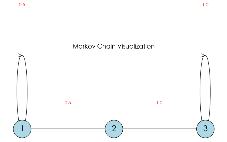
在上面的 3 状态系统 ($S=\{1, 2, 3\}$)中:
- 状态 1: 有 50% 概率留在他自己这里 ($1 \to 1$),有 50% 概率跳到 状态 2 ($1 \to 2$)。
- 状态 2: 100% 概率跳到 状态 3 ($2 \to 3$)。
- 状态 3: 100% 概率留在他自己这里 ($3 \to 3$)。
其中,
- 状态 1
- 它可以到达状态 2 ($1 \to 2$)。
- 瞬态 (Transient)。虽然它有 50% 的概率暂时留下,但从长远来看,它最终肯定会溜进状态 2,并且一旦离开,就再也没有路可以回去了。
- 非本质 (Inessential)。因为状态 2 不能回到状态 1,也就是说存在一个“有去无回”的路。
- 状态 2
- 它可以到达状态 3 ($2 \to 3$)
- 瞬态 (Transient)。它只能到达状态 3,并且一旦离开,就再也没有路可以回去了。
- 非本质 (Inessential)。因为状态 3 不能回到状态 2,也就是说存在一个“有去无回”的路。
- 状态 3
- 它只能到达它自己。
- 常返态 (Recurrent),也是吸收态 (Absorbing State)。
- 自己当然能回到自己,没有“泄露”到任何回不来的地方,所以它是 本质 (Essential) 的。
链的结构性质 (Structural Properties)
不可约性 (Irreducibility)
在这个链中,任意一个状态出发,都有可能(经过一步或多步)到达任意另一个状态。
- 数学符号: 对任意 $i, j \in S$,都有 $i \leftrightarrow j$(互通)。
- 直观理解: 整个系统是一个紧密的整体,没有被隔离的孤岛。
- 通俗理解: 如果一个城市称之为不可约,这意味着这个城市极其通畅。无论你现在在哪(比如状态 $i$),也无论你想去哪(比如状态 $j$),你总能找到一条路过去(可能需要换乘几次,也就是经过几步,但一定能到)。
可约 (Reducible): 这意味着城市里有“陷阱”或者“单行道区域”。一旦你进入了某个区域,就再也无法回到原来的地方了。系统被分成了不同的“阶级”或“部分”。
import networkx as nx
import matplotlib.pyplot as plt

def draw_chain(transitions, title, ax):
    G = nx.DiGraph()
    # 添加边和权重
    for u, v, p in transitions:
        G.add_edge(u, v, weight=p)

    # 使用圆形布局
    pos = nx.circular_layout(G)

    # 画节点
    nx.draw_networkx_nodes(G, pos, ax=ax, node_size=2000, node_color='lightblue', edgecolors='black')
    nx.draw_networkx_labels(G, pos, ax=ax, font_size=16, font_weight='bold')

    # 画边 (带弧度,避免重叠)
    nx.draw_networkx_edges(G, pos, ax=ax, arrowstyle='->', arrowsize=25,
                           connectionstyle='arc3, rad=0.15')

    # 标注概率
    edge_labels = {(u, v): f"{p}" for u, v, p in transitions}
    nx.draw_networkx_edge_labels(G, pos, edge_labels=edge_labels, ax=ax, label_pos=0.3, font_size=12)

    ax.set_title(title, fontsize=14)
    ax.axis('off')

# --- 1. 定义可约链 (Reducible) ---
# 这里的 "3" 是个死胡同 (吸收态),回不到 "1" 或 "2"
transitions_reducible = [
    (1, 1, 0.5),
    (1, 2, 0.5),
    (2, 3, 1.0),
    (3, 3, 1.0)
]

# --- 2. 定义不可约链 (Irreducible) ---
# 我们添加了 3->1,形成闭环,所有状态互通
transitions_irreducible = [
    (1, 1, 0.5),
    (1, 2, 0.5),
    (2, 3, 1.0),
    (3, 1, 1.0)
]

# --- 绘图 ---
fig, axes = plt.subplots(1, 2, figsize=(12, 5))

draw_chain(transitions_reducible, "Reducible (Broken Flow)", axes[0])
draw_chain(transitions_irreducible, "Irreducible (Connected Flow)", axes[1])

plt.tight_layout()
plt.show()
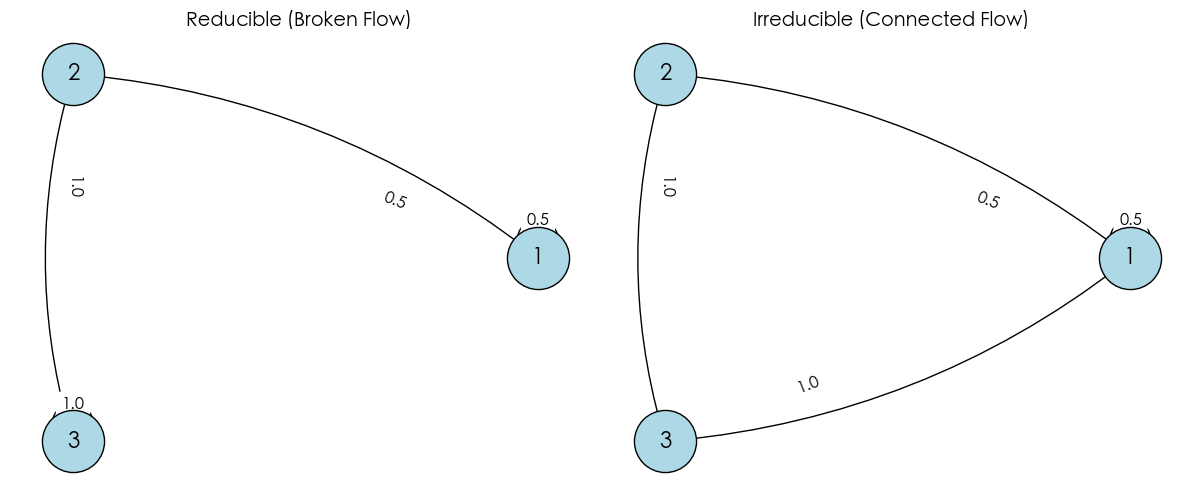
在上面的图中:
- 左图 (可约, Reducible): 包含一个“陷阱”(状态 3),一旦进去就回不到起点了。
- 右图 (不可约, Irreducible): 也就是刚才我们“手术”修复后的版本(添加 $3 \to 1$),所有状态互通。
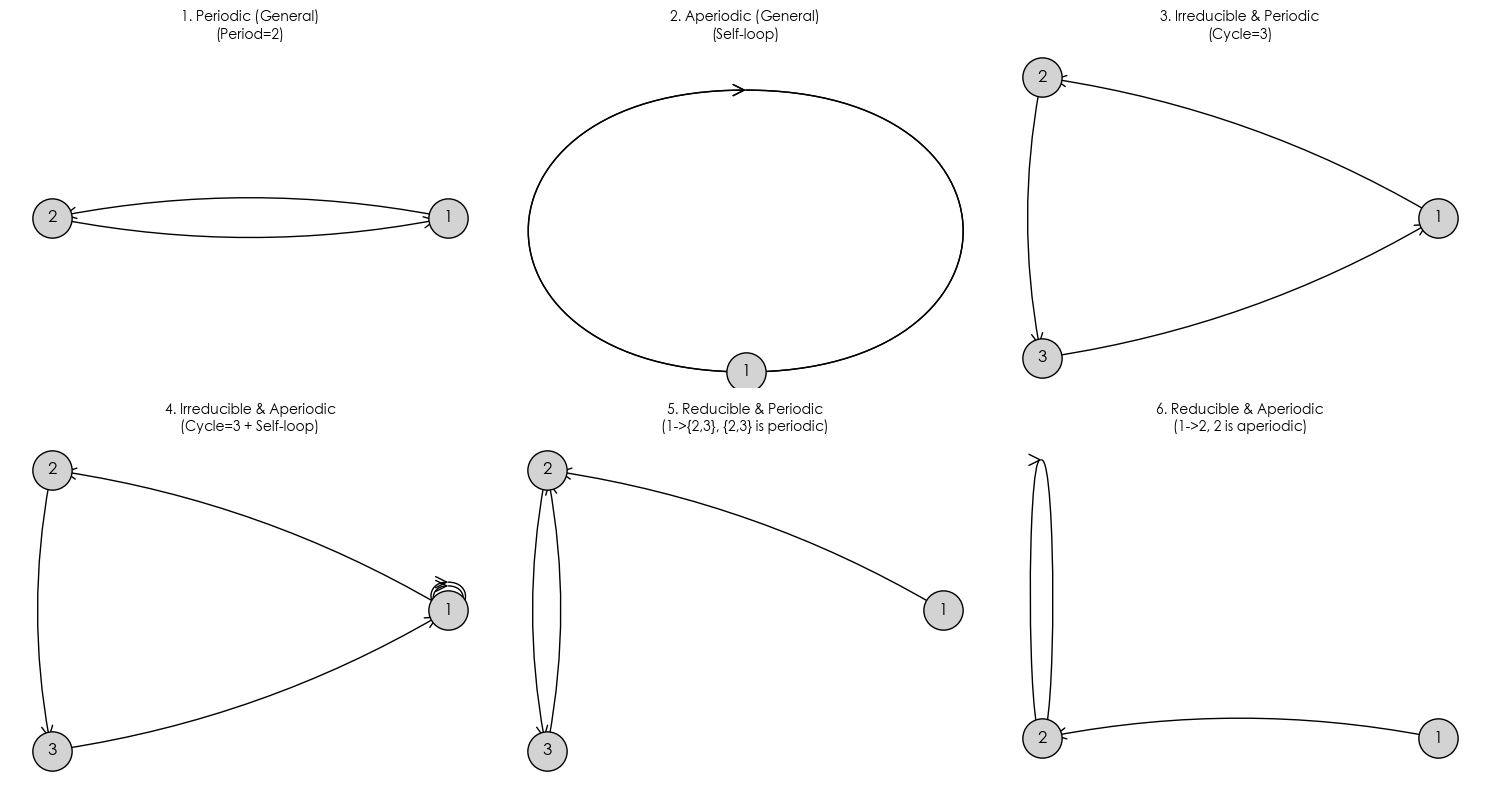
周期性 (Periodicity)
周期性描述的是系统回到原状态的“节奏感”。如果必须经过固定的步数(比如偶数步)才能回家,那它就是有周期的。
数学定义:对于状态 $i$,我们将所有能够让系统从 $i$ 出发并回到 $i$(即 $p_{ii}^{(n)} > 0$)的步数 $n$ 收集起来,构成一个集合:
$$ I_i = \{ n \ge 1 \mid p_{ii}^{(n)} > 0 \} $$状态 $i$ 的周期 $d(i)$ 定义为这个集合中所有数的最大公约数 (Greatest Common Divisor, GCD):
$$ d(i) = \text{gcd}(I_i) $$- 周期性 (Periodic): 如果 $d(i) > 1$,则称状态 $i$ 是周期的。
- 这里的 $d(i)$ 就是周期
- 非周期性 (Aperiodic): 如果 $d(i) = 1$,则称状态 $i$ 是非周期的。
- 也就是说,步数集合的公约数只能是 1。
- 只要状态 $i$ 有一个自环(Self-loop, $p_{ii} > 0$),它就是非周期的。这意味着你可以 1 步回来。那么 $1$ 就在集合 $I_i$ 里。包含 1 的集合,其最大公约数必然是 1。所以该状态是非周期的。
“不可约”可以是“周期性”的,也可以是非周期的。
在一个不可约马尔可夫链中,所有状态的周期都是相同的。也就是说,如果链中有一个状态是非周期的,那么整个链都是非周期的。
import networkx as nx
import matplotlib.pyplot as plt

def draw_subplot(transitions, title, ax, pos_type='circular'):
    G = nx.DiGraph()
    for u, v in transitions:
        G.add_edge(u, v)

    if pos_type == 'circular':
        pos = nx.circular_layout(G)
    else:
        pos = nx.spring_layout(G, seed=42) # 固定种子以保持形状

    # 绘制节点和边
    nx.draw_networkx_nodes(G, pos, ax=ax, node_size=800, node_color='lightgray', edgecolors='black')
    nx.draw_networkx_labels(G, pos, ax=ax, font_size=12, font_weight='bold')

    # 绘制带箭头的边 (使用arc3弯曲,防止重叠)
    nx.draw_networkx_edges(G, pos, ax=ax, arrowstyle='->', arrowsize=20,
                           connectionstyle='arc3, rad=0.1')

    # 检查是否有自环 (Self-loop),手动标记一下方便观察
    self_loops = list(nx.selfloop_edges(G))
    if self_loops:
        nx.draw_networkx_edges(G, pos, ax=ax, edgelist=self_loops,
                               arrowstyle='->', arrowsize=20, connectionstyle='arc3, rad=0.5')

    ax.set_title(title, fontsize=10)
    ax.axis('off')

# --- 定义六种情况 ---

# 1. 简单的周期性 (Periodic)
# 最简单的一来一回,周期为 2
t_periodic = [(1, 2), (2, 1)]

# 2. 简单的非周期性 (Aperiodic)
# 只要有自环,立刻打破周期,周期为 1
t_aperiodic = [(1, 1)]

# 3. 不可约 & 周期性 (Irreducible & Periodic)
# 一个大环,大家互通(不可约),但步数必须是 3 的倍数(周期 3)
t_irr_per = [(1, 2), (2, 3), (3, 1)]

# 4. 不可约 & 非周期性 (Irreducible & Aperiodic)
# 大家互通(不可约),但在 1 处加了个自环,节奏乱了(非周期)
t_irr_aper = [(1, 2), (2, 3), (3, 1), (1, 1)]

# 5. 可约 & 周期性 (Reducible & Periodic)
# 1 去 2 回不来(可约)。2 和 3 互跳(周期 2)。
# 注意:这里指 recurrent class {2,3} 是周期的。
t_red_per = [(1, 2), (2, 3), (3, 2)]

# 6. 可约 & 非周期性 (Reducible & Aperiodic)
# 1 去 2 回不来(可约)。2 有自环(非周期)。
t_red_aper = [(1, 2), (2, 2)]

# --- 绘图 ---
fig, axes = plt.subplots(2, 3, figsize=(15, 8))
axes = axes.flatten()

draw_subplot(t_periodic, "1. Periodic (General)\n(Period=2)", axes[0])
draw_subplot(t_aperiodic, "2. Aperiodic (General)\n(Self-loop)", axes[1])
draw_subplot(t_irr_per, "3. Irreducible & Periodic\n(Cycle=3)", axes[2])
draw_subplot(t_irr_aper, "4. Irreducible & Aperiodic\n(Cycle=3 + Self-loop)", axes[3])
draw_subplot(t_red_per, "5. Reducible & Periodic\n(1->{2,3}, {2,3} is periodic)", axes[4])
draw_subplot(t_red_aper, "6. Reducible & Aperiodic\n(1->2, 2 is aperiodic)", axes[5])

plt.tight_layout()
plt.show()
HIA Chain
HIA Chain 是马尔可夫链中的“黄金标准”。它同时满足这三个条件时:
- H (Homogeneous - 齐次性): 转移规则 $P$ 永远不变。
- I (Irreducible - 不可约性): 整个系统是连通的,没有死胡同。
- A (Aperiodic - 非周期性): 没有固定的循环节奏。
HIA 链的渐近行为 (Asymptotic Behavior)
假设
$$P = \begin{bmatrix} 0.7 & 0.3 \\ 0.4 & 0.6 \end{bmatrix}$$- 第一天 ($t=1, P^1$):$$\begin{bmatrix}
0.7 & 0.3 \\
0.4 & 0.6
\end{bmatrix}$$
- 此时两行差别很大:今天晴和今天雨,对明天的影响截然不同
- 第五天 ($t=5, P^5$):$$\begin{bmatrix}
0.5725 & 0.4275 \\
0.5700 & 0.4300
\end{bmatrix}$$
- 注意看,这两行的数字是不是开始变得有点像了?
- 第二十天 ($t=20, P^{20}$):$$\begin{bmatrix}
0.5714 & 0.4286 \\
0.5714 & 0.4286
\end{bmatrix}$$
- 这里可以看出,20 天前的初始天气对现在的预测已经没有影响了
HIA 链的极限定理 (Limit Theorem)
对于一个 HIA(齐次、不可约、非周期)的马尔可夫链,如果它的转移矩阵是 $P$,那么当步数 $n$ 趋向于无穷大时,会有如下结论:
$$\lim_{n \to \infty} p_{ij}^{(n)} = \pi_j$$这里的符号含义是:
- $p_{ij}^{(n)}$:表示从状态 $i$ 出发,经过 $n$ 步后,到达状态 $j$ 的概率。
- $\pi_j$:表示状态 $j$ 的 稳态概率(它是一个常数,与起始状态 $i$ 无关)。
矩阵形式如下:
$$ \lim_{n \to \infty} P^n = \begin{bmatrix} \pi_0 & \pi_1 & \dots & \pi_k \ \pi_0 & \pi_1 & \dots & \pi_k \ \vdots & \vdots & \ddots & \vdots \ \pi_0 & \pi_1 & \dots & \pi_k \end{bmatrix} $$- 行行相同: 最终矩阵的每一行都是完全一样的。
- 每一行都是 $\pi$: 每一行都是那个唯一的稳态分布向量 $\pi = [\pi_0, \pi_1, \dots, \pi_k]$。
- 遗忘初值: 无论你是从第 1 行(状态 0)出发,还是从第 $k$ 行(状态 $k$)出发,你最终停留在某个状态的概率都是一样的。
平稳分布 (Stationary Distribution)
定义:一个概率向量 $\pi$,如果
$$ \pi P = \pi, \quad \sum_i \pi_i = 1, \; \pi_i \geq 0 $$那么 $\pi$ 称为该马尔可夫链的 平稳分布。
意义:如果链在某个时刻的分布是 $\pi$,那么在之后任意时刻仍然保持 $\pi$。它描述了 长期状态分布。
混合时间 (Mixing Time)
收敛速度的度量
定义:链从初始分布 $\mu$ 到接近平稳分布所需的时间。
常用距离:全变差距离 (total variation distance)
$$ d(t) = \max_\mu \| \mu P^t - \pi \|_{TV} $$混合时间:最小 $t$,使得 $d(t) \leq \epsilon$。
遍历定理 (Ergodic Theorem)
定理: 对一个有限马尔可夫链,如果它是 不可约 且 非周期,则存在唯一平稳分布 $\pi$,并且:
$$ \lim_{n \to \infty} P(X_n = j \mid X_0 = i) = \pi_j \quad \forall i,j $$同时,时间平均收敛到概率平均:
$$ \frac{1}{N}\sum_{t=1}^N \mathbf{1}_{\{X_t=j\}} \to \pi_j $$通俗解释:你长期停留在某个状态的时间比例,恰好等于该状态的稳态概率。
$$Time Average = Space Average(时间平均 = 空间平均)$$这在实际应用中价值连城!这意味着我们不需要去解复杂的方程组求 $\pi$,只需要让计算机模拟“跑”一遍(蒙特卡洛模拟),数数它在每个坑里呆了多久,就能反推出 $\pi$。
可逆马尔可夫链 (Reversible Markov Chain)
一个马尔可夫链 $X = \{X_n\}$ 被称为 可逆 HIA 链 (Reversible HIA Chain),必须同时满足以下所有条件:
- 基础结构条件 (HIA)。首先,它必须是一个 HIA 链,这意味着:
- 齐次性 (Homogeneous): 转移矩阵 $P$ 是恒定的,不随时间 $t$ 变化。
- 不可约性 (Irreducible): 状态空间 $S$ 中任意两个状态都是互通的。
- 非周期性 (Aperiodic): 状态的重访步数没有固定的周期限制(即 $\text{gcd}(I_i) = 1$)。
- 可逆性条件 (Reversibility)。该链的平稳分布 $\pi$ 和转移矩阵 $P$ 必须满足 细致平衡方程 (Detailed Balance Equation): $$\pi_i P_{ij} = \pi_j P_{ji}, \quad \forall i, j \in S$$
满足条件一保证了该链存在唯一的 平稳分布 (Stationary Distribution) $\pi$。
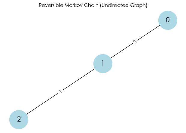
示例
import numpy as np
import networkx as nx
import matplotlib.pyplot as plt

# 1. 定义一个无向图 (Undirected Graph)
# 这里的权重 (weight) 可以理解为两个状态之间的“亲密度”或“通道宽窄”
G = nx.Graph()
G.add_edge(0, 1, weight=2)
G.add_edge(1, 2, weight=1)

# 2. 自动构建转移矩阵 P
# 规则:从节点 i 跳到邻居 j 的概率 = (i,j的权重) / (i 的所有权重之和)
nodes = sorted(G.nodes())
n = len(nodes)
P = np.zeros((n, n))

for i in nodes:
    total_weight = sum([G[i][nbr]['weight'] for nbr in G.neighbors(i)])
    for j in G.neighbors(i):
        P[i, j] = G[i][j]['weight'] / total_weight

print("--- 转移矩阵 P ---")
print(P)

# 3. 计算稳态分布 pi
# 技巧:对于无向图,pi_i 正比于节点 i 的“度” (所有连接边的权重和)
degrees = [sum([G[i][nbr]['weight'] for nbr in G.neighbors(i)]) for i in nodes]
total_degree_sum = sum(degrees)
pi = np.array([d / total_degree_sum for d in degrees])

print("\n--- 稳态分布 pi ---")
print(f"pi = {pi}")

# 4. 验证细致平衡 (Detailed Balance): pi_i * P_ij = pi_j * P_ji ?
print("\n--- 验证细致平衡 (Flow Check) ---")
# 检查 状态 0 <-> 状态 1
flow_0_to_1 = pi[0] * P[0, 1]
flow_1_to_0 = pi[1] * P[1, 0]

print(f"Flow 0 -> 1: {pi[0]:.4f} * {P[0, 1]:.4f} = {flow_0_to_1:.4f}")
print(f"Flow 1 -> 0: {pi[1]:.4f} * {P[1, 0]:.4f} = {flow_1_to_0:.4f}")

if np.isclose(flow_0_to_1, flow_1_to_0):
    print("✅ 状态 0 和 1 之间满足细致平衡!")
else:
    print("❌ 不平衡")

# --- 绘图 ---
pos = nx.spring_layout(G, seed=42)
plt.figure(figsize=(6, 4))
nx.draw(G, pos, with_labels=True, node_color='lightblue', node_size=2000, font_size=16)
labels = nx.get_edge_attributes(G, 'weight')
nx.draw_networkx_edge_labels(G, pos, edge_labels=labels)
plt.title("Reversible Markov Chain (Undirected Graph)")
plt.show()
--- 转移矩阵 P ---
[[0.         1.         0.        ]
 [0.66666667 0.         0.33333333]
 [0.         1.         0.        ]]

--- 稳态分布 pi ---
pi = [0.33333333 0.5        0.16666667]

--- 验证细致平衡 (Flow Check) ---
Flow 0 -> 1: 0.3333 * 1.0000 = 0.3333
Flow 1 -> 0: 0.5000 * 0.6667 = 0.3333
✅ 状态 0 和 1 之间满足细致平衡!
细致平衡 vs. 全局平衡
细致平衡(局部) $\implies$ 全局平衡。证明如下。
证明 $\pi$ 满足全局平衡方程:
$$\sum_{i} \pi_i P_{ij} = \pi_j$$- 出发: 看等式左边 $\sum_{i} \pi_i P_{ij}$。
- 代入: 利用细致平衡 ($\pi_i P_{ij} = \pi_j P_{ji}$),把 $\pi_i P_{ij}$ 换成 $\pi_j P_{ji}$。$$\sum_{i} (\pi_j P_{ji})$$
- 提取: 把常数 $\pi_j$ 提到求和符号外面。$$\pi_j \sum_{i} P_{ji}$$
- 归一: 因为 $P$ 是转移矩阵,从状态 $j$ 出发去往所有可能状态 $i$ 的概率之和必须为 1 ($\sum_{i} P_{ji} = 1$)。$$\pi_j \times 1 = \pi_j$$
- 结论: 左边等于右边。证毕!✅
可逆 HIA 链的渐近分布
“可逆 HIA 链的渐近分布” (Asymptotic distribution of reversible HIA Chains) 描述的是:当时间趋于无穷大时,一个性质非常特殊的马尔可夫链最终会稳定在什么样的状态。
- HIA 链 (HIA Chains):这是 齐次 (Homogeneous)、不可约 (Irreducible) 且 非周期 (Aperiodic) 的马尔可夫链的缩写。
- 这就好比一个永远在洗牌的机器,规则不变,所有牌都能洗到,而且没有固定的节奏。
- 重点: HIA 链保证了无论你从哪里开始,经过足够长的时间(渐近行为,$n \to \infty$),系统处于各个状态的概率都会收敛到一个固定的值。
- 渐近分布 (Asymptotic Distribution):这就是上面提到的“固定的值”。也就是当 $n$ 趋近于无穷大时,状态分布 $\pi_n$ 的极限。
- 在 HIA 链中,这个渐近分布就是我们常说的 平稳分布 (Stationary Distribution, $\pi$)。
- 它满足方程:$\pi = \pi P$(全局平衡方程)。
- 可逆性 (Reversible):这是最特殊的“魔法调料”。如果一个 HIA 链是可逆的,它的平稳分布 $\pi$ 会满足一个更严格、更简单的条件,叫做 细致平衡 (Detailed Balance):$$\pi_i P_{ij} = \pi_j P_{ji}$$
- 这意味着:在稳态下,从状态 $i$ 跳到 $j$ 的“流量”,完全等于从 $j$ 跳回 $i$ 的“流量”。
所谓的“可逆 HIA 链的渐近分布”,其实就是利用细致平衡方程 ($\pi_i P_{ij} = \pi_j P_{ji}$) 求出的那个唯一的平稳分布 $\pi$。
示例
import numpy as np
import matplotlib.pyplot as plt

# ============ 基础工具 ============

def is_row_stochastic(P, tol=1e-12):
    """检查转移矩阵是否“行随机”(每行和约为1,元素>=0)"""
    P = np.asarray(P, dtype=float)
    nonneg = np.all(P >= -tol) # 检查非负性
    rowsum_one = np.allclose(P.sum(axis=1), 1.0, atol=1e-10) # 检查每行和是否约为1
    return bool(nonneg and rowsum_one), P.sum(axis=1)

def n_step_transition(P, n):
    """n 步转移矩阵:P^n"""
    return np.linalg.matrix_power(np.asarray(P, dtype=float), n)

def simulate_markov_chain(P, init_state, n_steps, rng=None):
    """
    从单个初始状态模拟一条马尔可夫链路径。
    P: 行随机矩阵;init_state: int (0..S-1);返回数组 shape=(n_steps+1,)
    """
    if rng is None:
        rng = np.random.default_rng()
    P = np.asarray(P, dtype=float)
    S = P.shape[0] # 状态数
    path = np.empty(n_steps+1, dtype=int) # 初始化路径
    path[0] = int(init_state) # 确保初始状态是整数
    for t in range(n_steps): # 逐步生成路径
        i = path[t]
        path[t+1] = rng.choice(S, p=P[i]) # 从当前状态 i 选择下一个状态
    return path

def simulate_many(P, pi0, n_steps, n_runs=10000, rng=None):
    """
    模拟多条路径,估计各时刻的经验分布(与理论 pi0 P^t 对比)。
    返回:
      emp_dist: shape=(n_steps+1, S) 经验分布
      th_dist : shape=(n_steps+1, S) 理论分布
    """
    if rng is None:
        rng = np.random.default_rng()
    P = np.asarray(P, dtype=float)
    S = P.shape[0]
    # 理论分布随时间演化
    th = np.zeros((n_steps+1, S))
    th[0] = pi0
    for t in range(n_steps):
        th[t+1] = th[t] @ P
    # 经验分布
    counts = np.zeros((n_steps+1, S), dtype=int)
    init_states = rng.choice(S, size=n_runs, p=pi0)
    for r in range(n_runs):
        s0 = init_states[r]
        path = simulate_markov_chain(P, s0, n_steps, rng=rng)
        for t in range(n_steps+1):
            counts[t, path[t]] += 1
    emp = counts / n_runs
    return emp, th
示例 1:两状态(天气示例:晴=S,雨=R)
模型设定(两状态天气链)
状态:0=晴 (Sunny),1=雨 (Rainy) 转移矩阵:
$$ P=\begin{bmatrix} \text{晴→晴} & \text{晴→雨}\\ \text{雨→晴} & \text{雨→雨} \end{bmatrix}=\begin{bmatrix} 0.8 & 0.2\\ 0.4 & 0.6 \end{bmatrix} $$含义:晴→晴 0.8、晴→雨 0.2;雨→晴 0.4、雨→雨 0.6。
- 行随机:每行和为 1(合法概率矩阵)。
- 不可约:每个状态都能到达另一个状态(两行都含非零对向转移)。
- 非周期:对角元 $p_{00},p_{11}>0$(有自环),周期为 1。 ⇒ 链是遍历的(ergodic):存在唯一平稳分布,且从任意初值都会收敛到它。
# ============ 示例 1:两状态(晴/雨) ============
# 状态编码:0=晴(S), 1=雨(R)
P2 = np.array([[0.8, 0.2],
[0.4, 0.6]], dtype=float)
ok, rowsums = is_row_stochastic(P2)
print("P2 行随机性检查:", ok, " 行和=", rowsums)
# 单一路径模拟与可视化
rng = np.random.default_rng(2025)
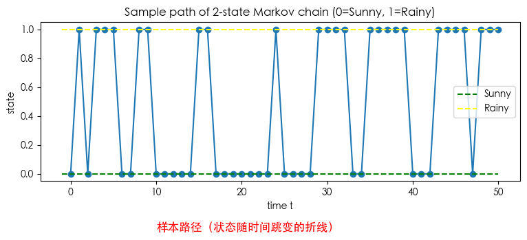
path = simulate_markov_chain(P2, init_state=0, n_steps=50, rng=rng)
plt.figure(figsize=(9,3))
plt.plot(range(len(path)), path, marker='o')
plt.hlines(0, -1, len(path)-1, colors='green', linestyles='dashed', label="Sunny")
plt.hlines(1, -1, len(path)-1, colors='yellow', linestyles='dashed', label="Rainy")
plt.text(10, -0.4, "样本路径(状态随时间跳变的折线)", fontsize=12, color='red')
plt.title("Sample path of 2-state Markov chain (0=Sunny, 1=Rainy)")
plt.xlabel("time t")
plt.ylabel("state")
plt.legend()
plt.show()
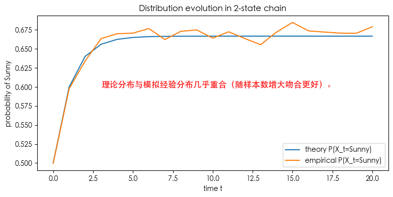
# 多路径统计 vs 理论分布
pi0 = np.array([0.5, 0.5]) # 初始分布
emp, th = simulate_many(P2, pi0, n_steps=20, n_runs=5000, rng=rng)
# 画“处于 Sunny 的概率”随时间变化:理论 vs 经验
plt.figure(figsize=(9,4))
plt.plot(th[:,0], label="theory P(X_t=Sunny)")
plt.plot(emp[:,0], label="empirical P(X_t=Sunny)")
plt.text(3, 0.6, "理论分布与模拟经验分布几乎重合(随样本数增大吻合更好)。", fontsize=12, color='red')
plt.title("Distribution evolution in 2-state chain")
plt.xlabel("time t")
plt.ylabel("probability of Sunny")
plt.legend()
plt.show()
# n 步转移矩阵示例
P2_5 = n_step_transition(P2, 5)
print("P2^5 =\n", np.round(P2_5, 4))
P2 行随机性检查: True 行和= [1. 1.]
P2^5 =
 [[0.6701 0.3299]
 [0.6598 0.3402]]
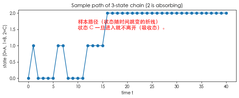
示例 2:三状态(含吸收态 C)
$$ P_3= \begin{bmatrix} 0.6 & 0.4 & 0.0\\ 0.2 & 0.5 & 0.3\\ 0.0 & 0.0 & 1.0 \end{bmatrix}, $$# ============ 示例 2:三状态(含吸收态 C) ============
# 状态编码:0=A, 1=B, 2=C(吸收)
P3 = np.array([[0.6, 0.4, 0.0],
[0.2, 0.5, 0.3],
[0.0, 0.0, 1.0]], dtype=float)
ok3, rowsums3 = is_row_stochastic(P3)
print("P3 行随机性检查:", ok3, " 行和=", rowsums3)
path3 = simulate_markov_chain(P3, init_state=0, n_steps=40, rng=rng)
plt.figure(figsize=(9,3))
plt.plot(range(len(path3)), path3, marker='o')
plt.text(10, 1.5, "样本路径(状态随时间跳变的折线)\n状态 C 一旦进入就不离开(吸收态)。", fontsize=12, color='red')
plt.title("Sample path of 3-state chain (2 is absorbing)")
plt.xlabel("time t")
plt.ylabel("state (0=A, 1=B, 2=C)")
plt.show()
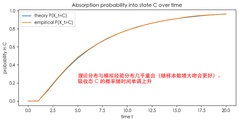
# 多路径统计:观测吸收到 C 的概率随时间变化
pi0_3 = np.array([1.0, 0.0, 0.0]) # 从 A 起步
emp3, th3 = simulate_many(P3, pi0_3, n_steps=20, n_runs=5000, rng=rng)
plt.figure(figsize=(9,4))
plt.plot(th3[:,2], label="theory P(X_t=C)")
plt.plot(emp3[:,2], label="empirical P(X_t=C)")
plt.text(5, 0.2, "理论分布与模拟经验分布几乎重合(随样本数增大吻合更好)。\n吸收态 C 的概率随时间单调上升", fontsize=12, color='red')
plt.title("Absorption probability into state C over time")
plt.xlabel("time t")
plt.ylabel("probability in C")
plt.legend()
plt.show()
# n 步转移矩阵示例
P3_5 = n_step_transition(P3, 5)
print("P3^5 =\n", np.round(P3_5, 4))
P3 行随机性检查: True 行和= [1. 1. 1.]
P3^5 =
 [[0.242  0.2856 0.4724]
 [0.1428 0.1706 0.6866]
 [0.     0.     1.    ]]
示例
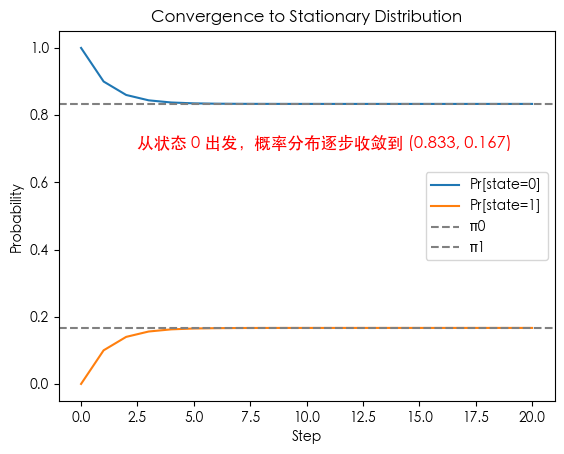
示例 1:两状态马尔可夫链
最简单的演示,清晰看到收敛到平稳分布。
转移矩阵:
$$ P = \begin{bmatrix} 0.9 & 0.1 \\ 0.5 & 0.5 \end{bmatrix} $$(a) 平稳分布
解方程:
$$ \pi P = \pi $$即:
$$ \pi_0 = 0.9\pi_0 + 0.5\pi_1 \quad\Rightarrow\quad 0.1\pi_0 = 0.5\pi_1 $$结合 $\pi_0 + \pi_1 = 1$,解得:
$$ \pi = (0.833..., \; 0.166...) $$(b) 性质分析
- 不可约。因为两个状态互相可达(两行都含非零对向转移)。
- 非周期:因为 $P_{00}>0, P_{11}>0$(有自环),可保持在原状态 → 周期 = 1
综上,根据遍历定理,该有限马尔可夫链是遍历的(ergodic),即存在唯一平稳分布,且从任意初值都会收敛到它。
(c) 收敛过程
import numpy as np
import matplotlib.pyplot as plt

P = np.array([[0.9, 0.1],
              [0.5, 0.5]])

# 初始分布
mu = np.array([1.0, 0.0])

distributions = [mu]
for _ in range(20):
    mu = mu @ P
    distributions.append(mu)

distributions = np.array(distributions)

plt.plot(distributions[:,0], label="Pr[state=0]")
plt.plot(distributions[:,1], label="Pr[state=1]")
plt.axhline(0.833, color="gray", linestyle="--", label="π0")
plt.axhline(0.167, color="gray", linestyle="--", label="π1")
plt.text(2.5, 0.7, "从状态 0 出发,概率分布逐步收敛到 (0.833, 0.167)", fontsize=12, color='red')
plt.xlabel("Step")
plt.ylabel("Probability")
plt.legend()
plt.title("Convergence to Stationary Distribution")
plt.show()
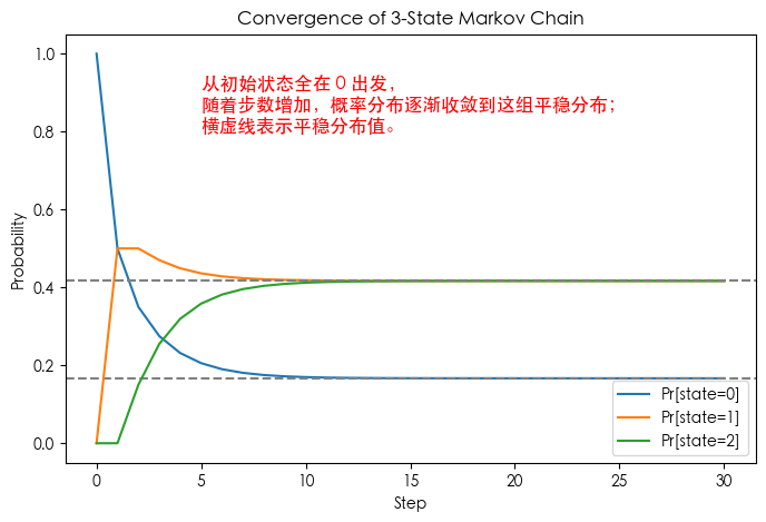
示例 2:三状态马尔可夫链
展示了更复杂链中平稳分布的存在性和唯一性。
转移矩阵:
$$ P = \begin{bmatrix} 0.5 & 0.5 & 0.0 \\ 0.2 & 0.5 & 0.3 \\ 0.0 & 0.3 & 0.7 \end{bmatrix} $$- 不可约:所有状态可互相到达。
- 非周期:存在自循环概率 $P_{ii} > 0$。
- 平稳分布:解 $\pi P = \pi$,得到唯一 $\pi$。
- 长期行为:所有初始分布都会收敛到 $\pi$。
import numpy as np
import matplotlib.pyplot as plt

# 三状态马尔可夫链转移矩阵
P = np.array([[0.5, 0.5, 0.0],
              [0.2, 0.5, 0.3],
              [0.0, 0.3, 0.7]])

# 初始分布(全部在状态0)
mu = np.array([1.0, 0.0, 0.0])

# 计算平稳分布:解 pi P = pi
eigvals, eigvecs = np.linalg.eig(P.T)
stat_dist = eigvecs[:, np.isclose(eigvals, 1)]
stat_dist = stat_dist[:,0]
stat_dist = stat_dist / stat_dist.sum()  # 归一化
print("Stationary distribution:", stat_dist.real)

# 迭代分布演化
distributions = [mu]
for _ in range(30):
    mu = mu @ P
    distributions.append(mu)

distributions = np.array(distributions)

# 绘图
plt.figure(figsize=(8,5))
for i in range(3):
    plt.plot(distributions[:, i], label=f"Pr[state={i}]")
    plt.axhline(stat_dist[i].real, linestyle="--", color="gray")

plt.text(5, 0.8, "从初始状态全在 0 出发,\n随着步数增加,概率分布逐渐收敛到这组平稳分布;\n横虚线表示平稳分布值。", fontsize=12, color='red')
plt.xlabel("Step")
plt.ylabel("Probability")
plt.title("Convergence of 3-State Markov Chain")
plt.legend()
plt.show()
Stationary distribution: [0.16666667 0.41666667 0.41666667]
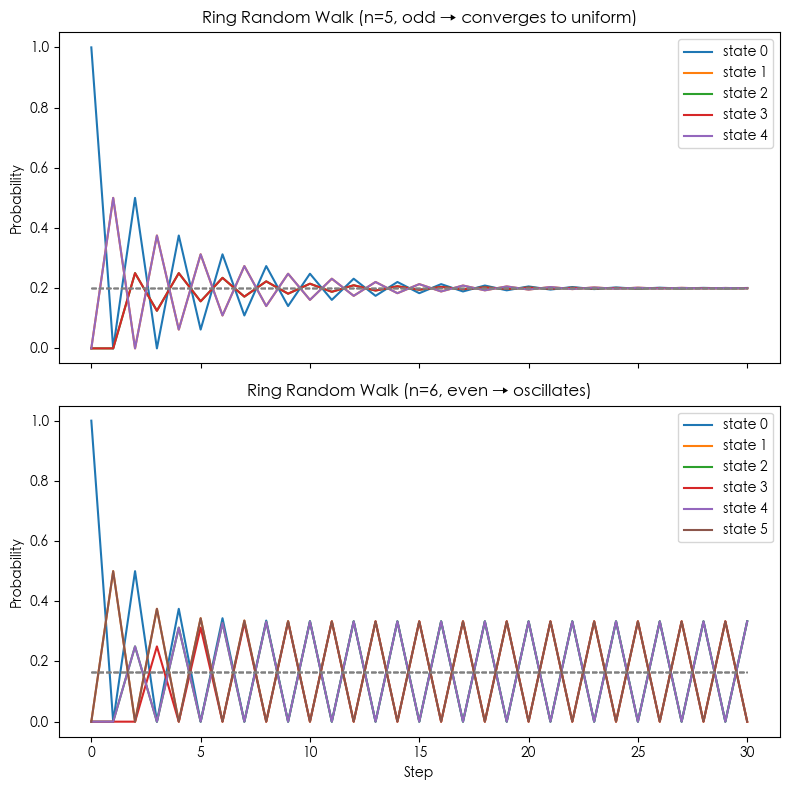
示例 3:环形随机游走 (Random Walk on a Cycle)
展示了 周期性 对收敛性的影响。
状态:$\{0,1,2,\dots,n-1\}$。
转移规则:从当前位置 $i$,以概率 0.5 移动到 $(i−1)\bmod n$,以概率 0.5 移动到 $(i+1)\bmod n$。即
$$ P(i \to i+1 \bmod n) = 0.5, \quad P(i \to i-1 \bmod n) = 0.5 $$不可约:从任意状态可到任意状态。
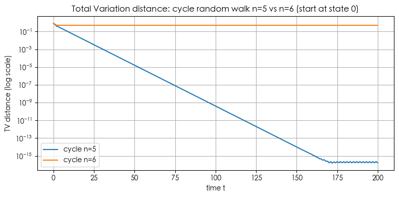
周期性:如果 $n$ 是偶数,则周期 = 2;如果 $n$ 是奇数,则非周期。
平稳分布:均匀分布 $\pi_i = 1/n$。
收敛性:
- 若 $n$ 奇数 → 链是不可约且非周期 → 收敛到均匀分布。
- 若 $n$ 偶数 → 链有周期性(周期=2) → 链会在“奇数/偶数类”之间来回跳,无法收敛到均匀分布。
import numpy as np
import matplotlib.pyplot as plt

def ring_rw_transition_matrix(n):
    """生成 n 状态的环形随机游走转移矩阵"""
    P = np.zeros((n, n))
    for i in range(n):
        P[i, (i-1)%n] = 0.5
        P[i, (i+1)%n] = 0.5
    return P

def simulate_chain(P, steps=30, start_state=0):
    """从单点分布开始,计算分布演化"""
    n = P.shape[0]
    mu = np.zeros(n)
    mu[start_state] = 1.0
    distributions = [mu]
    for _ in range(steps):
        mu = mu @ P
        distributions.append(mu)
    return np.array(distributions)

# 参数
steps = 30
P5 = ring_rw_transition_matrix(5)
P6 = ring_rw_transition_matrix(6)

# 模拟
dist5 = simulate_chain(P5, steps)
dist6 = simulate_chain(P6, steps)

# 平稳分布(对于奇数 n,均匀分布;偶数情况不存在唯一收敛)
pi5 = np.ones(5) / 5
pi6 = np.ones(6) / 6

# 绘图
fig, axes = plt.subplots(2, 1, figsize=(8,8), sharex=True)

# n=5
for i in range(5):
    axes[0].plot(dist5[:, i], label=f"state {i}")
axes[0].hlines(pi5, 0, steps, colors="gray", linestyles="--", linewidth=1)
axes[0].set_title("Ring Random Walk (n=5, odd → converges to uniform)")
axes[0].set_ylabel("Probability")
axes[0].legend()

# n=6
for i in range(6):
    axes[1].plot(dist6[:, i], label=f"state {i}")
axes[1].hlines(pi6, 0, steps, colors="gray", linestyles="--", linewidth=1)
axes[1].set_title("Ring Random Walk (n=6, even → oscillates)")
axes[1].set_xlabel("Step")
axes[1].set_ylabel("Probability")
axes[1].legend()

plt.tight_layout()
plt.show()
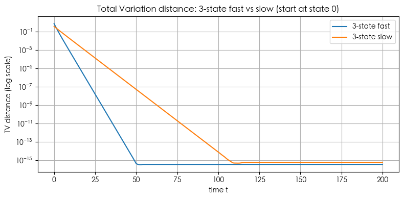
示例 4: 混合时间 (Mixing Time) 的数值度量(比如 total variation distance 收敛速度)
# Simulate Markov chains and compute total variation distance (TV) to the stationary distribution.
# We will:
# 1. Define several transition matrices (fast/slow 3-state, cycle random walks n=5 and n=6).
# 2. Compute TV distance over time starting from state 0.
# 3. Compute mixing times tau(epsilon) for epsilons = [0.1, 0.01, 0.001].
# 4. Plot TV vs time for comparisons and show a table of mixing times.
#
# Note: Plots use matplotlib (no seaborn) and each figure is a single plot as requested.

import numpy as np
import pandas as pd
import matplotlib.pyplot as plt

def stationary_from_P(P):
    # solve pi = pi P  with sum(pi)=1  -> transpose eigenvector of P^T for eigenvalue 1
    w, v = np.linalg.eig(P.T)
    idx = np.argmin(np.abs(w - 1.0))
    pi = np.real(v[:, idx])
    pi = pi / pi.sum()
    pi = np.maximum(pi, 0)
    pi = pi / pi.sum()
    return pi

def tv_distance(p, q):
    return 0.5 * np.sum(np.abs(p - q))

def tv_curve(P, p0, t_max):
    n = P.shape[0]
    pis = stationary_from_P(P)
    p = p0.copy()
    tvs = []
    for t in range(t_max + 1):
        tvs.append(tv_distance(p, pis))
        p = p @ P
    return np.array(tvs), pis

def mixing_time_from_tvs(tvs, eps):
    # minimal t such that tvs[t] <= eps
    below = np.where(tvs <= eps)[0]
    return int(below[0]) if below.size > 0 else np.nan

# Define chains
# 3-state fast chain
P_fast = np.array([
    [0.6, 0.3, 0.1],
    [0.2, 0.6, 0.2],
    [0.1, 0.3, 0.6]
])

# 3-state slow chain (more "sticky" on state 0)
P_slow = np.array([
    [0.9, 0.08, 0.02],
    [0.2, 0.7, 0.1],
    [0.15, 0.15, 0.7]
])

# Cycle random walk
def cycle_P(n):
    P = np.zeros((n, n))
    for i in range(n):
        P[i, (i+1) % n] = 0.5
        P[i, (i-1) % n] = 0.5
    return P

P_cycle5 = cycle_P(5)
P_cycle6 = cycle_P(6)

# initial distribution: start at state 0
def e0(n):
    v = np.zeros(n); v[0]=1.0; return v

t_max = 200

# compute tv curves
tvs_fast, pi_fast = tv_curve(P_fast, e0(3), t_max)
tvs_slow, pi_slow = tv_curve(P_slow, e0(3), t_max)

tvs_c5, pi_c5 = tv_curve(P_cycle5, e0(5), t_max)
tvs_c6, pi_c6 = tv_curve(P_cycle6, e0(6), t_max)

# compute mixing times for selected epsilons
epsilons = [1e-1, 1e-2, 1e-3]
rows = []
for name, tvs in [
    ("3-state fast", tvs_fast),
    ("3-state slow", tvs_slow),
    ("cycle n=5", tvs_c5),
    ("cycle n=6", tvs_c6)
]:
    entry = {"chain": name}
    for eps in epsilons:
        entry[f"tau({eps})"] = mixing_time_from_tvs(tvs, eps)
    rows.append(entry)

df_mix = pd.DataFrame(rows)

# Plot 1: 3-state fast vs slow
plt.figure(figsize=(8,4))
plt.plot(tvs_fast, label='3-state fast')
plt.plot(tvs_slow, label='3-state slow')
plt.yscale('log')  # show both fast and slow clearly on log scale
plt.xlabel('time t')
plt.ylabel('TV distance (log scale)')
plt.title('Total Variation distance: 3-state fast vs slow (start at state 0)')
plt.legend()
plt.grid(True)
plt.tight_layout()
plt.show()

# Plot 2: cycle n=5 vs n=6
plt.figure(figsize=(8,4))
plt.plot(tvs_c5, label='cycle n=5')
plt.plot(tvs_c6, label='cycle n=6')
plt.yscale('log')
plt.xlabel('time t')
plt.ylabel('TV distance (log scale)')
plt.title('Total Variation distance: cycle random walk n=5 vs n=6 (start at state 0)')
plt.legend()
plt.grid(True)
plt.tight_layout()
plt.show()


# Also print stationary distributions for reference
pi_table = pd.DataFrame({
    "chain": ["3-state fast", "3-state slow", "cycle n=5", "cycle n=6"],
    "stationary": [pi_fast, pi_slow, pi_c5, pi_c6]
})
pi_table['stationary_str'] = pi_table['stationary'].apply(lambda x: np.array2string(x, precision=4, separator=', '))
pi_table = pi_table[['chain','stationary_str']]
display("Stationary distributions", pi_table)
'Stationary distributions'
| chain | stationary_str | |
|---|---|---|
| 0 | 3-state fast | [0.2857, 0.4286, 0.2857] |
| 1 | 3-state slow | [0.6466, 0.2328, 0.1207] |
| 2 | cycle n=5 | [0.2, 0.2, 0.2, 0.2, 0.2] |
| 3 | cycle n=6 | [0.1667, 0.1667, 0.1667, 0.1667, 0.1667, 0.1667] |
Scan to Share
微信扫一扫分享