Stochastic Optimization
In an environment full of uncertainty (noise) or extreme complexity (non-convexity), how do we use “randomness” to find the best solution?
From Deterministic to Stochastic Optimization
Problem Definition: Starting from the Deterministic World
It all starts with a classic optimization puzzle. Minimize a system’s state, described mathematically as:
$$\min_{x \in Q} E(x) = m$$Where:
- $x$ is the parameter we are looking for (e.g., model weights, molecular configuration).
- $E(x)$ is our energy function (called Loss Function in machine learning). The goal is to make it as small as possible.
- $m$ is the theoretical global minimum.
In the world of Deterministic Methods, we usually move step by step along the gradient direction, like a blind person walking down a hill. This is effective in simple terrains (convex functions), but in complex real-world problems, we easily get trapped in “pits” of local optima.
Welcome to Stochastic World
To escape the trap of local optima, we use a key transformation: We convert the problem of “finding minimum energy” into “finding maximum probability”.
This transformation is based on the Boltzmann Distribution in physics. We define a new probability density function (PDF):
$$f(x) = A e^{-E(x)}$$Where:
- $f(x)$: Probability density function, must be positive.
- $A = \frac{1}{\int e^{-E(x)} \, dx}$ is the Normalization Constant.
- In statistical physics, the reciprocal of $A$ has a famous name: Partition Function, usually denoted by $Z$. $$Z = \frac{1}{A} = \int e^{-E(x)} \, dx$$
There is an ingenious correspondence here:
- The smaller $E(x)$ (lower energy, which is what we want).
- The larger $e^{-E(x)}$.
- This means the minimum point of $E(x)$ corresponds exactly to the peak (maximum) of the probability distribution $f(x)$.
Thus, the original problem corresponds to:
$$\min E(x) \iff \max f(x)$$Why make this transformation?
Because in the stochastic world, we are no longer obsessed with “going down every step”, but view the solution space as a probability field. We allow the algorithm to accept “bad results” with a certain probability, and it is this mechanism that gives us the opportunity to jump out of local traps.
Introducing Temperature Parameter $\lambda$
To control the search process, we introduce a crucial parameter $\lambda$. So the probability density function becomes:
$$f(x, \lambda) = A_\lambda e^{-\lambda E(x)}$$Where $\lambda$ is positive and inversely proportional to temperature $T$:
$$\lambda = \frac{1}{T} \ge 0$$Thus, $A$ becomes $A = \frac{1}{\int e^{-\lambda E(x)} \, dx}$
This $\lambda$ (or $T$) acts like a regulator, determining the “resolution” or “contrast” of the terrain. We can change the shape of the probability distribution $f(x, \lambda)$ by adjusting it.
Two Extreme States: Exploration and Exploitation
By analyzing the limit cases of $\lambda$, we can perfectly reveal the mechanism of stochastic optimization:
State A: High Temperature Mode
When $\lambda \to 0$ (meaning $T \to \infty$):
- Mathematically: $-\lambda E(x) \to 0$, leading to $e^{-\lambda E(x)} \to 1$.
- Result: $f(x, \lambda) \to \text{Constant}$.
- Physical Picture: The probability distribution tends to be uniform throughout the space. Regardless of $E(x)$, the probability of sampling any point is almost equal.
- Significance: This is the Exploration phase. The algorithm moves violently in space like gas molecules, easily crossing any high mountains and deep valleys, ensuring we don’t miss the region where the global optimum is located.
State B: Low Temperature Mode
When $\lambda \to \infty$ (meaning $T \to 0$):
- Mathematically: Differences are amplified infinitely. As long as $E(x)$ is slightly larger, $e^{-\lambda E(x)}$ decays extremely fast.
- Result: The probability distribution becomes a sharp peak (similar to a Dirac $\delta$ function), having value only at the lowest energy point $m$.
- Physical Picture: The system “freezes”.
- Significance: This is the Exploitation phase. The algorithm locks onto the lowest point of the current region and stops running around, thus obtaining a high-precision solution.
import numpy as np
import matplotlib.pyplot as plt
from matplotlib.animation import FuncAnimation, PillowWriter

# --- 1. Define Energy Function ---
# We design an asymmetric double well:
# A deep pit (global optimum), a shallow pit (local optimum)
def energy_function(x):
    # (x^2 - 1)^2 is standard W-shaped double well
    # + 0.3*x tilts it, making the left pit deeper than the right
    return (x**2 - 1)**2 + 0.3 * x

# --- 2. Prepare Data ---
x = np.linspace(-2.5, 2.5, 500)
E = energy_function(x)

# Find true global min for plotting
min_idx = np.argmin(E)
global_min_x = x[min_idx]
global_min_y = E[min_idx]

# --- 3. Setup Plot ---
fig, (ax1, ax2) = plt.subplots(2, 1, figsize=(8, 10), constrained_layout=True)

# Top: Energy Landscape E(x) - Static
ax1.plot(x, E, 'k-', linewidth=3, label='Energy $E(x)$')
ax1.scatter(global_min_x, global_min_y, color='gold', s=150, zorder=5, edgecolors='k', label='Global Min')
ax1.set_title("The Problem: Energy Landscape $E(x)$", fontsize=14)
ax1.set_ylabel("Energy")
ax1.grid(True, alpha=0.3)
ax1.legend()
ax1.set_xlim(-2.5, 2.5)

# Bottom: Probability Distribution f(x) - Changes with T
line, = ax2.plot([], [], 'r-', linewidth=3, alpha=0.8)
fill_poly = ax2.fill_between(x, np.zeros_like(x), np.zeros_like(x), color='red', alpha=0.3)
ax2.set_xlim(-2.5, 2.5)
ax2.set_ylabel("Probability Density $f(x)$")
ax2.set_xlabel("x")
ax2.grid(True, alpha=0.3)

# Dynamic Text: Lambda and Temperature
text_info = ax2.text(0.05, 0.9, '', transform=ax2.transAxes, fontsize=12,
                     bbox=dict(facecolor='white', alpha=0.8))

# --- 4. Animation Logic ---
# Lambda from 0.1 (High T) to 15.0 (Low T)
# Log scale to show high T phase slowly, low T phase quickly
lambdas = np.logspace(np.log10(0.1), np.log10(15.0), 100)

def init():
    line.set_data([], [])
    return line,

def update(frame_lambda):
    global fill_poly

    # === Core Physics ===
    # 1. Boltzmann Factor (Unnormalized Prob)
    # e^(-lambda * E)
    unnormalized_prob = np.exp(-frame_lambda * E)

    # 2. Normalization Constant A (Partition Function Z)
    # Numerical integration using trapezoidal rule
    integral_Z = np.trapezoid(unnormalized_prob, x)
    A = 1.0 / integral_Z

    # 3. Final PDF f(x)
    # f(x) = A * e^(-lambda * E)
    pdf = A * unnormalized_prob
    # =================

    # Update curve
    line.set_data(x, pdf)

    # Update fill (remove old, add new)
    fill_poly.remove()
    fill_poly = ax2.fill_between(x, 0, pdf, color='red', alpha=0.3)

    # Dynamically adjust Y limit (peaks get higher)
    ax2.set_ylim(0, np.max(pdf) * 1.2)

    # Update title and text
    T = 1 / frame_lambda
    ax2.set_title(f"The Stochastic Solution: Probability Distribution", fontsize=14)
    text_info.set_text(f"$\lambda$ = {frame_lambda:.2f} (Inverse Temp)\n$T$ = {T:.2f} (Temperature)")

    return line, fill_poly, text_info

# --- 5. Generate and Save ---
print("Generating animation...")
ani = FuncAnimation(fig, update, frames=lambdas, init_func=init, blit=False)

# Save as GIF
ani.save('simulated_annealing.gif', writer=PillowWriter(fps=15))
print("✅ Saved as 'simulated_annealing.gif'")
This is a classic “Double Well” energy function:
- It has a global optimum (deep pit).
- And a local optimum (shallow pit).
At high temperatures, the probability distribution covers both pits; as temperature drops ($\lambda$ increases), the probability distribution gradually “abandons” the local optimum and squeezes entirely into the “peak” of the global optimum.
From MCMC to Optimization: The Art of Annealing (The Bridge: Simulated Annealing)
Simulated Annealing (SA) is a general probabilistic optimization algorithm.
- Name Origin: From the “annealing” process in metallurgy.
- Physical Annealing: Heat metal to high temp (atoms move freely), then cool slowly. Atoms have time to find the lowest energy crystal structure, making metal hard and defect-free.
- Algorithmic Annealing: Throw parameter $x$ into high temp (random walk), then slowly lower $T$. $x$ has time to escape local optima and settle in global optimum.
- Core Feature: It is an algorithm that “allows regret”. During search, it accepts not only “good” solutions but also “bad” solutions with some probability (to jump out of pits).
Steepest Descent mentioned before is “snobbish”, only going downhill. If the terrain is like an egg carton (countless small pits), gradient descent dies in the first pit it falls into.
SA’s advantages:
- Global Search Capability: Because it accepts “bad solutions” at high T, it can climb over hills to explore unknown territories.
- Gradient-Free: No derivatives needed ($f(x)$ can even be discontinuous).
- Versatile: Works on any ugly function as long as you can calculate the value.
- Applicable even if $f(x)$ is non-convex.
Algorithm Flow
- Transform: We don’t solve $\min E(x)$ directly, but construct a probability distribution: $$f(x) \propto e^{-E(x)/T}$$
- Here $\lambda = 1/T$.
- Intuition: Turn “terrain height” into “probability density”. Deeper pit ($E$ small) -> higher probability. Higher mountain ($E$ large) -> lower probability.
- High Temperature Exploration (High T Sampling):
- Action: Set a high initial temperature $T_{max}$.
- Phenomenon:
- When $T$ is large, $E(x)/T \approx 0$, so $e^0 \approx 1$.
- The whole probability distribution is Flat, close to uniform.
- Your “particle” (sample) will run around the map (since probability of going anywhere is similar), easily crossing mountains and escaping local traps.
- Cooling / Annealing: Slowly lower temperature $T$ (increase $\lambda$).
- Action: Lower $T$ according to a schedule.
- Theoretical: $T(t) \sim \frac{c}{\log(1+t)}$ (Guarantees global opt, but strictly slow).
- Practical: $T_{new} = T_{old} \times \alpha$.
- $\alpha$: Cooling Rate, usually between $0.8$ and $0.99$.
- Phenomenon: As T drops, distribution “deforms”. Flat areas get lower, deep pits get deeper (peaks get sharper).
- Action: Lower $T$ according to a schedule.
- Low Temperature Exploitation: Loop till Low T.
- Action: Continue “Sample -> Cool -> Sample” until $T$ is very low.
- ⚠️ But not 0, or division is undefined.
- Phenomenon: Probability distribution becomes a needle (Dirac Delta). Particle is essentially “locked” in the deepest pit.
- Action: Continue “Sample -> Cool -> Sample” until $T$ is very low.
- Sample & Average:
- Action: Collect samples $x_1, \dots, x_n$ at low temp stage, calculate their mean.
- Conclusion: This mean $\bar{x}$ is our estimated global minimum $x_{min}$.
Note:
- At first $T$ is huge, $\Delta E / T$ small, $P$ near 1. Algorithm accepts almost all bad moves (Crazy run).
- Later $T$ is tiny, $\Delta E / T$ huge, $P$ near 0. Algorithm rejects almost all bad moves (Becomes gradient descent).
Examples
1D Example
Using a function with multiple traps to show “Temperature Control” + “Metropolis Sampling”: $E(x) = x^2 - \cos(\pi x)$.
import numpy as np
import matplotlib.pyplot as plt

# --- 1. Objective Function ---
def E(x):
    return x**2 - np.cos(np.pi * x)

# --- 2. Sampling Core: Metropolis Criterion ---
# This is a "sampler", generates sample based on current T
def sample_one_step(x_curr, T):
    # a. Propose: Random step left or right
    x_next = x_curr + np.random.uniform(-0.5, 0.5)

    # b. Delta E
    dE = E(x_next) - E(x_curr)

    # c. Accept/Reject
    # Core Logic: If new energy is lower, go; if higher, go with prob (depends on T)
    if dE < 0 or np.random.rand() < np.exp(-dE / T):
        return x_next # Accept
    else:
        return x_curr # Reject

# --- Main Flow ---
def run_stochastic_optimization():
    x = -2.5       # Start (Deliberately far local opt)
    T = 10.0       # T_max
    T_min = 0.01   # T_min
    alpha = 0.99   # Cooling rate

    path = []
    temps = []

    print(f"{'Step':<6} | {'Temp':<8} | {'Current x':<10} | {'Action'}")
    print("-" * 45)

    step = 0
    # Flow 4: Till very low T
    while T > T_min:

        # Flow 2 & 3: Sample & Cool
        x = sample_one_step(x, T)

        path.append(x)
        temps.append(T)

        # Print intermediate
        if step % 200 == 0:
            status = "Explore 🎲" if T > 1.0 else "Exploit 🎯"
            print(f"{step:<6} | {T:<8.4f} | {x:<10.4f} | {status}")

        T = T * alpha
        step += 1

    # Flow 5: Avg Samples
    final_samples = path[-100:]
    estimated_min = np.mean(final_samples)

    print("-" * 45)
    print(f"✅ Final Estimate: x = {estimated_min:.4f}")
    print(f"✅ True Min: x = 0.0000")

    return path, temps

# --- Run & Visualize ---
path, temps = run_stochastic_optimization()

plt.figure(figsize=(10, 6))
plt.plot(path, alpha=0.6, label='Particle Path')
plt.xlabel('Iterations (Time)')
plt.ylabel('Position x')
plt.title('Algorithm Flow: From Exploration (High T) to Exploitation (Low T)')
plt.axhline(0, color='r', linestyle='--', label='Global Min (x=0)')
plt.grid(True, alpha=0.3)
plt.legend()
plt.show()
Step   | Temp     | Current x  | Action
---------------------------------------------
0      | 10.0000  | -2.5000    | Explore 🎲
200    | 1.3398   | 1.6236     | Explore 🎲
400    | 0.1795   | 0.2889     | Exploit 🎯
600    | 0.0241   | 0.0178     | Exploit 🎯
---------------------------------------------
✅ Final Estimate: x = -0.0050
✅ True Min: x = 0.0000
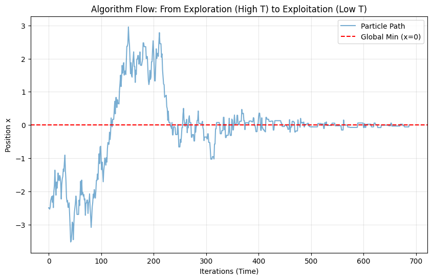
Graph Analysis:
- First half (Left): Curve oscillates violently. High temp exploration, particle doesn’t care about pits, jumping everywhere.
- Second half (Right): Curve becomes a straight line. Low temp locking, particle trapped near $x=0$.
- Result: Averaging the “static” points at the end gives precise minimum.
N-Dimensional Example
Using the famous Rastrigin Function. It’s notorious: macroscopically a bowl (global opt exists), microscopically full of pits (egg carton).
Formula ($A=10$):
$$f(\mathbf{x}) = 10n + \sum_{i=1}^n (x_i^2 - 10 \cos(2\pi x_i))$$Global min at origin $\mathbf{x} = [0, \dots, 0]$, value 0.
import numpy as np
import matplotlib.pyplot as plt

# --- 1. N-D Objective (Rastrigin) ---
def rastrigin(x):
    # x is vector
    A = 10
    n = len(x)
    return A * n + np.sum(x**2 - A * np.cos(2 * np.pi * x))

# --- 2. N-D Proposal ---
def get_neighbor(x_curr, step_size=0.5):
    # Key: Random walk in N-D space
    # size=len(x_curr) ensures dimension match
    perturbation = np.random.uniform(-step_size, step_size, size=len(x_curr))
    return x_curr + perturbation

# --- 3. Simulated Annealing Main ---
def simulated_annealing_nd(n_dim=2, n_iter=2000):
    # Init: Random start in range [-5.12, 5.12]
    current_x = np.random.uniform(-5.12, 5.12, size=n_dim)
    current_E = rastrigin(current_x)

    # Track Best So Far
    best_x = current_x.copy()
    best_E = current_E

    # Temps
    T = 100.0
    T_min = 1e-4
    alpha = 0.99

    path = [current_x]
    energy_history = [current_E]

    print(f"Start {n_dim}-D Optimization...")
    print(f"Start: {np.round(current_x, 2)}, Energy: {current_E:.2f}")

    iter_count = 0
    while T > T_min and iter_count < n_iter:
        # 1. Propose
        new_x = get_neighbor(current_x)
        new_x = np.clip(new_x, -5.12, 5.12) # Clip to domain

        new_E = rastrigin(new_x)

        # 2. Delta E
        dE = new_E - current_E

        # 3. Metropolis Criterion
        if dE < 0 or np.random.rand() < np.exp(-dE / T):
            current_x = new_x
            current_E = new_E

            if current_E < best_E:
                best_x = current_x.copy()
                best_E = current_E

        path.append(current_x)
        energy_history.append(current_E)

        T *= alpha
        iter_count += 1

    print(f"End. Final Loc: {np.round(best_x, 4)}")
    print(f"Final Energy: {best_E:.6f} (Theoretical 0.0)")

    return np.array(path), energy_history, best_x

# --- Run ---
DIMENSION = 2
path, energies, final_sol = simulated_annealing_nd(n_dim=DIMENSION, n_iter=3000)

# --- 4. Visualize (2D only) ---
if DIMENSION == 2:
    plt.figure(figsize=(12, 5))

    # Subplot 1: Terrain & Path
    plt.subplot(1, 2, 1)
    x_grid = np.linspace(-5.12, 5.12, 100)
    y_grid = np.linspace(-5.12, 5.12, 100)
    X, Y = np.meshgrid(x_grid, y_grid)
    Z = np.zeros_like(X)
    for i in range(X.shape[0]):
        for j in range(X.shape[1]):
            Z[i,j] = rastrigin(np.array([X[i,j], Y[i,j]]))

    plt.contourf(X, Y, Z, levels=50, cmap='viridis', alpha=0.7)
    plt.colorbar(label='Energy')

    # Path: White start, Red end
    plt.plot(path[:, 0], path[:, 1], 'w-', linewidth=0.5, alpha=0.6)
    plt.scatter(path[0, 0], path[0, 1], c='white', s=50, label='Start')
    plt.scatter(final_sol[0], final_sol[1], c='red', marker='*', s=200, label='End')
    plt.legend()
    plt.title(f"2D Rastrigin Optimization Path\n(Escaping many local minima)")

    # Subplot 2: Energy Drop
    plt.subplot(1, 2, 2)
    plt.plot(energies)
    plt.yscale('log')
    plt.xlabel('Iteration')
    plt.ylabel('Energy (Log Scale)')
    plt.title('Energy Minimization Process')
    plt.grid(True, which="both", ls="--")

    plt.tight_layout()
    plt.show()
Start 2-D Optimization...
Start: [-2.9 -2.5], Energy: 36.46
End. Final Loc: [-0.0686 -0.9187]
Final Energy: 3.039640 (Theoretical 0.0)
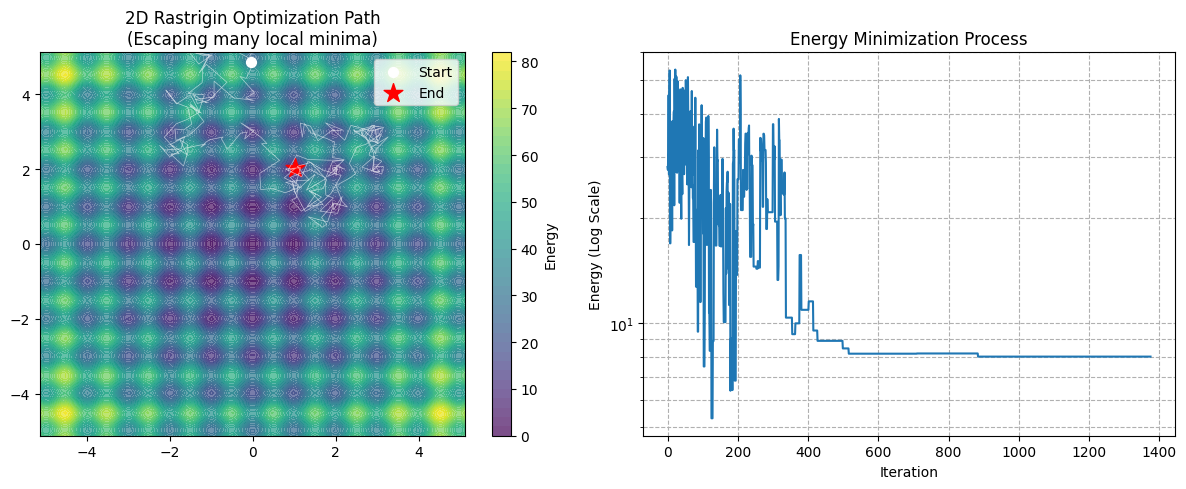
- Key code:
perturbation = np.random.uniform(-step_size, step_size, size=len(x_curr)). This is the core of N-D extension. We generate an N-D random vector at once. - Terrain (Left): Many deep blue circles, each is a local trap.
- Gradient Descent: Likely falls into the nearest blue circle and dies.
- Simulated Annealing: White path scurries around (especially early on). Jumps in, jumps out, until T drops, sucked into the middle deepest pit (Red Star).
Proof of Correctness: Pincus Theorem
Pincus Theorem provides the Theoretical Guarantee for SA convergence.
Pincus Theorem (Mark Pincus, 1968)
Pincus Theorem is a bridge proving: When we lower T to extremely low ($\lambda \to \infty$), the “weighted average” (expectation) of a function converges to its “global minimum point”.
It turns an “Optimization Problem” into an “Integration Problem”.
Assume objective $f(x)$ on domain $D$, global min $x^*$. Pincus Theorem states:
$$x^* = \lim_{\lambda \to \infty} \frac{\int_D x \cdot e^{-\lambda f(x)} \, dx}{\int_D e^{-\lambda f(x)} \, dx}$$Or in expectation form:
$$x^* = \lim_{\lambda \to \infty} \mathbb{E}_{\lambda}[x]$$Proof
Goal: Limit of fraction:
$$\langle x \rangle_\lambda = \frac{\int x \cdot e^{-\lambda E(x)} \, dx}{\int e^{-\lambda E(x)} \, dx}$$Prove finding $x^*$.
Step 1: Extract “Greatest Common Divisor”
Assume unique global min $x^*$. For any $x \neq x^*$, $E(x) > E(x^*)$.
Factor out $e^{-\lambda E(x^*)}$ from numerator and denominator.
- Denom: $\int e^{-\lambda E(x)} \, dx = e^{-\lambda E(x^*)} \int e^{-\lambda (E(x) - E(x^*))} \, dx$
- Num: $\int x e^{-\lambda E(x)} \, dx = e^{-\lambda E(x^*)} \int x \cdot e^{-\lambda (E(x) - E(x^*))} \, dx$
Substitute back, $e^{-\lambda E(x^*)}$ cancels out!
$$\langle x \rangle_\lambda = \frac{\int x \cdot e^{-\lambda (E(x) - E(x^*))} \, dx}{\int e^{-\lambda (E(x) - E(x^*))} \, dx}$$Now exponent is $-\lambda (E(x) - E(x^*))$. Note $\Delta E = E(x) - E(x^*) \ge 0$.
Step 2: Split Integration Domain (Neighborhood vs. Far Away)
Split domain into:
- Small neighborhood $U_\epsilon$ around min: $|x - x^*| < \epsilon$.
- Rest $R$: Far away.
As $\lambda \to \infty$:
- Region $R$: $\Delta E \ge \delta > 0$. Term $e^{-\lambda \Delta E} \le e^{-\lambda \delta}$. Decays exponentially to 0. Contributions from far regions are negligible.
- Neighborhood $U_\epsilon$: $\Delta E \approx 0$, so $e^{-\lambda \Delta E} \approx 1$. Integral dominated by this tiny region.
Step 3: Taylor Expansion
Near $x^*$:
$$E(x) \approx E(x^*) + E'(x^*)(x-x^*) + \frac{1}{2}E''(x^*)(x-x^*)^2$$Since $x^*$ is min, $E'(x^*) = 0$, $E''(x^*) = k > 0$.
$$E(x) - E(x^*) \approx \frac{1}{2} k (x-x^*)^2$$Substitute into integral (only neighborhood):
$$\text{Denom} \approx \int_{x^*-\epsilon}^{x^*+\epsilon} e^{-\lambda \frac{1}{2} k (x-x^*)^2} \, dx$$This is a Gaussian Integral. Recall $\int e^{-ax^2} dx = \sqrt{\frac{\pi}{a}}$, here $a = \frac{\lambda k}{2}$.
$$\text{Denom} \approx \sqrt{\frac{2\pi}{\lambda k}}$$Similarly for Numerator: $x \approx x^*$ is constant in small neighborhood.
$$ \text{Num} \approx x^* \cdot \sqrt{\frac{2\pi}{\lambda k}} $$Step 4: Cancellation
$$\lim_{\lambda \to \infty} \langle x \rangle_\lambda \approx \frac{x^* \cdot \sqrt{\frac{2\pi}{\lambda k}}}{\sqrt{\frac{2\pi}{\lambda k}}}$$Roots, $\pi$, derivative $k$, and $\lambda$ all cancel out! Remaining:
$$= x^*$$More Examples
This example is from the classroom.
This example is a classic optimization case study, demonstrating how to use the Simulated Annealing (SA) algorithm to find the global minimum of a multi-modal function (which has multiple local minima), and comparing it with a deterministic algorithm (Newton’s Method) to showcase the advantage of stochastic algorithms in complex terrains.
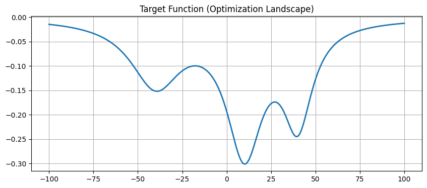
Defining the Target Function
We first define a function composed of the sum of three reciprocal quadratic functions:
$$ f(x) = \sum \frac{a_i}{b_i+(x+c_i)^2} $$- Geometric Meaning: This creates three main “pits” (local minima) on the graph.
- Challenge: One of them is the deepest (global optimum), while the other two are traps. If we only look at the slope under our feet (Gradient Descent / Newton’s Method), we can easily fall into a shallow pit and get stuck.
import numpy as np
import matplotlib.pyplot as plt

# ==========================================
# 1. Define Target Function
# ==========================================
# A constructed multi-modal function with multiple pits
def target_func(x):
    # Parameters (corresponding to a, b, c in formula)
    a = np.array([-40, -20, -40])
    b = np.array([150, 100, 300])
    c = np.array([-10, -40, 40])

    y = 0
    for i in range(3):
        y += a[i] / (b[i] + (x + c[i])**2)
    return y

# Plot range
xmin, xmax = -100, 100
x_vec = np.linspace(xmin, xmax, 1000)
y_vec = target_func(x_vec)

plt.figure(figsize=(10, 4))
plt.plot(x_vec, y_vec, linewidth=2)
plt.title('Target Function (Optimization Landscape)')
plt.grid(True)
plt.show()
Temperature Law: The Soul of SA
This is simulation annealing’s most critical setting.
In Simulated Annealing, we map the target function value $E(x)$ (energy) to a probability $P(x)$. The mapping rule is the Boltzmann Distribution:
$$P(x) = \frac{1}{Z} \cdot e^{-\frac{E(x)}{T}}$$- $E(x)$: Energy (the target function value to minimize).
- $T$: Temperature.
- $Z$: Normalization constant.
Substituting into the Metropolis acceptance rate formula $\alpha = \min\left(1, \frac{P(\text{new})}{P(\text{old})}\right)$, the constant $Z$ cancels out, leaving:
$$P(\text{accept}) = \exp\left(-\frac{\Delta E}{T}\right)$$- $\Delta E = E(\text{new}) - E(\text{old})$: How much worse the energy became.
- $T$: Current temperature (tolerance).
This formula tells us: The higher the temperature $T$, the higher the tolerance, and the greater the probability $P$ of accepting a bad move.
We can reverse-engineer the temperature from this formula:
$$T = -\frac{\Delta E}{\ln(P)}$$Why calculate $T_{in}$ and $T_{end}$?
- Initial Temperature $T_{in}$: Set to allow an 80% probability ($P=0.8$) of accepting even the worst case (jumping from lowest to highest point). This ensures “High Exploration” so the particle can jump anywhere.
- $\Delta E$ value:
max(fx) - min(fx).
- $\Delta E$ value:
- Final Temperature $T_{end}$: Set to allow only a 5% probability ($P=0.05$) of accepting tiny fluctuations ($\Delta E = 10^{-3}$). This ensures “Low Exploitation” (freezing), locking onto the solution.
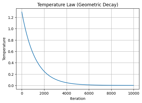
Geometric Cooling: $T(k) = T_{in} \cdot e^{-\tau k}$
Geometric Cooling is not a physical law but an engineering compromise to the theoretical “Logarithmic Cooling” (which is too slow).
Directly borrowing from Newton’s Law of Cooling: Reduce temperature by a fixed percentage each step.
$$T_{k+1} = \alpha \cdot T_k$$- $\alpha$: Cooling Rate, usually $0.8$ to $0.99$.
Expanding this gives the exponential decay form:
$$T(k) = T_0 \cdot e^{-\tau k}$$Where $\tau$ is the decay constant.
We can derive $\tau$ from boundary conditions:
- Start: $k=0, T=T_{in}$
- End: $k=i_{max}-1, T=T_{end}$
Solving for $\tau$:
$$\tau = -\frac{\ln(T_{end}/T_{in})}{i_{max} - 1}$$# ==========================================
# 2. Define Temperature Schedule
# ==========================================
# We want:
# - At Tin: 80% prob to accept max energy jump (High Exploration)
# - At Tend: 5% prob to accept tiny jump (1e-3) (High Locking)
y_max, y_min = np.max(y_vec), np.min(y_vec)
delta_E_max = y_max - y_min
# Reverse calculate T
# P = exp(-dE / T) => ln(P) = -dE / T => T = -dE / ln(P)
T_in = -delta_E_max / np.log(0.8)
T_end = -1e-3 / np.log(0.05)
n_iter = 10000
# Geometric Cooling: T(k) = T_in * exp(-tau * k)
# At k = n_iter-1, T = T_end
tau = -np.log(T_end / T_in) / (n_iter - 1)
iterations = np.arange(n_iter)
T_schedule = T_in * np.exp(-tau * iterations)
plt.figure(figsize=(6, 4))
plt.plot(iterations, T_schedule)
plt.title('Temperature Law (Geometric Decay)')
plt.xlabel('Iteration')
plt.ylabel('Temperature')
plt.grid(True)
plt.show()
Simulated Annealing Main Loop (Metropolis Core)
Inside the loop is standard Metropolis:
- Random Walk:
randn(1)*sd + sx(i-1). - Energy Check:
- If better ($\Delta E < 0$), accept ($>1$).
- If worse ($\Delta E > 0$), calculate $e^{-\Delta E/T}$.
- Key: Since $T$ decreases, the same bad move is forgiven (accepted) early on, but rejected later.
# ==========================================
# 3. Simulated Annealing Main Loop
# ==========================================
print("Starting Simulated Annealing...")
sx = np.zeros(n_iter)
alpha_hist = np.zeros(n_iter)
# Initial Point (Random)
current_x = np.random.randn() * 10
sx[0] = current_x
proposal_std = 50 # Standard deviation for proposal
for i in range(1, n_iter):
# 1. Propose: Random Walk
# Truncated to constraints
while True:
candidate = current_x + np.random.randn() * proposal_std
if xmin <= candidate <= xmax:
break
# 2. Calculate Energy Diff
E_curr = target_func(current_x)
E_cand = target_func(candidate)
dE = E_cand - E_curr # Minimize
# 3. Acceptance Ratio
T_curr = T_schedule[i]
# alpha = exp(-dE / T)
alpha = min(1, np.exp(-dE / T_curr))
alpha_hist[i] = alpha
# 4. Accept/Reject
if np.random.rand() < alpha:
current_x = candidate
# else: keep current_x
sx[i] = current_x
# Result (Mean of last 20% samples)
t_burn = int(0.8 * n_iter)
x_sol_stochastic = np.mean(sx[t_burn:])
y_sol_stochastic = target_func(x_sol_stochastic)
print(f"Stochastic Solution (SA): x = {x_sol_stochastic:.4f}, y = {y_sol_stochastic:.4f}")
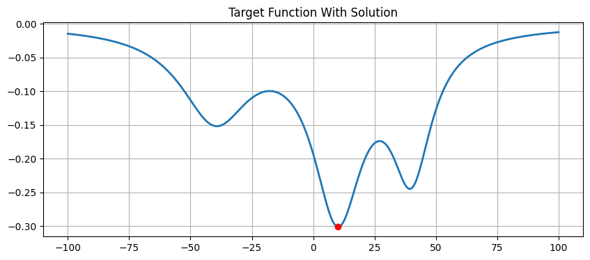
# Plot on the image
plt.figure(figsize=(10, 4))
plt.plot(x_vec, y_vec, linewidth=2)
plt.plot(x_sol_stochastic, y_sol_stochastic, 'ro')
plt.title('Target Function With Solution')
plt.grid(True)
plt.show()
Starting Simulated Annealing...
Stochastic Solution (SA): x = 10.0012, y = -0.3010
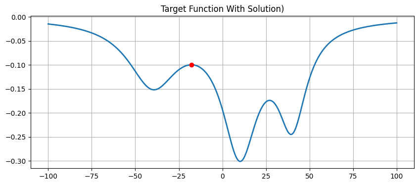
Contrast: Deterministic Algorithm (Newton’s Method)
We also implemented a simple Newton’s method for comparison.
- Principle: Uses second derivative information to fit a parabola to find extremums. Converges extremely fast.
- Outcome: We deliberately set the start point at $x=-10$.
- From the graph, $x=-10$ is near a local peak (maximum).
- Newton’s method is “myopic”; it sees a nearby peak and rushes up, unaware of the deeper pit further away.
- Conclusion: Newton’s method found a local optimum, while Simulated Annealing (due to early random jumps) successfully skipped this trap and found the global optimum.
# ==========================================
# 4. Deterministic Contrast (Newton's Method)
# ==========================================
# Newton: x_new = x - f'(x) / f''(x)
# Deliberately start far from global opt, near a local opt
x_newton = -10.0
newton_path = [x_newton]

# Central Difference for Derivatives
def get_derivatives(f, x, h=1e-5):
    # First derivative f'
    df = (f(x + h) - f(x - h)) / (2 * h)
    # Second derivative f''
    ddf = (f(x + h) - 2*f(x) + f(x - h)) / (h**2)
    return df, ddf

for _ in range(100):
    df, ddf = get_derivatives(target_func, x_newton)
    if abs(ddf) < 1e-6: break # Prevent div by zero

    step = df / ddf
    x_newton = x_newton - step
    newton_path.append(x_newton)

    if abs(step) < 1e-6: break # Converged

y_sol_deterministic = target_func(x_newton)
print(f"Deterministic Solution (Newton): x = {x_newton:.4f}, y = {y_sol_deterministic:.4f}")

# Plot on the image
plt.figure(figsize=(10, 4))
plt.plot(x_vec, y_vec, linewidth=2)
plt.plot(x_newton, y_sol_deterministic, 'ro')
plt.title('Target Function With Solution)')
plt.grid(True)
plt.show()
Deterministic Solution (Newton): x = -17.7557, y = -0.0996
Visual Comparison
# ==========================================
# 5. Final Visualization
# ==========================================
plt.figure(figsize=(12, 6))
plt.plot(x_vec, y_vec, label='Target Function', color='blue', alpha=0.5)

# Plot SA samples (color by time)
plt.scatter(sx[::10], target_func(sx[::10]), c=np.arange(0, n_iter, 10),
            cmap='Wistia', alpha=0.5, s=10, label='SA Trajectory')

# Mark Solutions
plt.plot(x_sol_stochastic, y_sol_stochastic, 'r*', markersize=20, label='SA Solution (Global)')
plt.plot(x_newton, y_sol_deterministic, 'kx', markersize=15, markeredgewidth=3, label='Newton Solution (Local)')

plt.colorbar(label='Iteration Time')
plt.legend()
plt.title('Global Optimization: Simulated Annealing vs Newton Method')
plt.xlim(xmin, xmax)
plt.show()
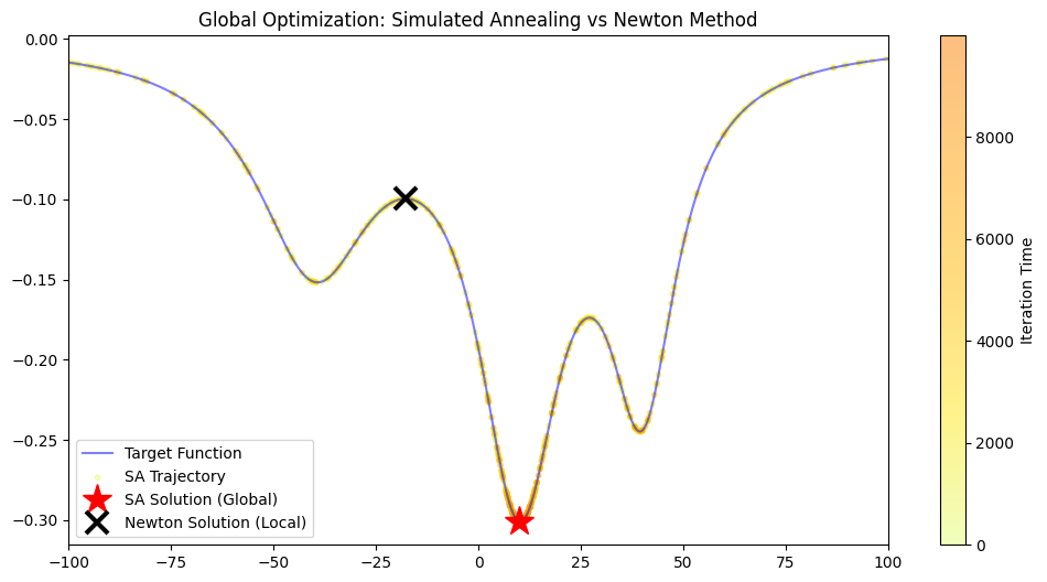
- Yellow/Orange dots: Footprints of SA. Lighter (early) dots are everywhere (exploring); darker (late) dots concentrate in the deepest pit.
- Red Star (SA): Landed accurately on the global minimum.
- Black Cross (Newton): Regrettably stuck on a nearby peak.
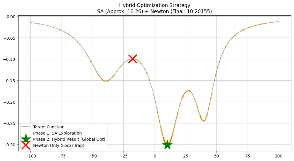
Hybrid Optimization
Using only one method has issues:
- Simulated Annealing only: Very inefficient at the end. To reduce error from 0.01 to 0.000001, you need to cool down extremely slowly, requiring millions of iterations. Like embroidery with a sledgehammer.
- Newton only: Unless you are lucky and start near the global optimum, it will likely fall into a local trap. Like finding a path with a microscope.
Solution: Combine them.
- Use SA to get an Approximate Global Solution.
- Low Precision, High Robustness. It jumps out of traps and lands near the hole.
- Use Newton to get the Exact Solution.
- High Precision, Fragile. Since SA already put it in the right “basin of attraction”, Newton will slide it into the hole at quadratic speed.
import numpy as np
import matplotlib.pyplot as plt

# Plot Prep
x_vec = np.linspace(-100, 100, 1000)
y_vec = target_func(x_vec)

# ==========================================
# Phase 1: Simulated Annealing (Global Search)
# ==========================================
print("🚀 Phase 1: Simulated Annealing (Global Search)...")

# 1. Auto Temp
y_max, y_min = np.max(y_vec), np.min(y_vec)
delta_E_max = y_max - y_min

# Init: 80% accept max jump; End: 5% accept tiny jump
T_in = -delta_E_max / np.log(0.8)
T_end = -1e-3 / np.log(0.05)

n_iter = 5000
tau = -np.log(T_end / T_in) / (n_iter - 1)

# Init
current_x = np.random.uniform(-90, 90) # Random Start
sx = np.zeros(n_iter)
proposal_std = 20

# SA Loop
for i in range(n_iter):
    T_curr = T_in * np.exp(-tau * i)

    while True:
        candidate = current_x + np.random.randn() * proposal_std
        if -100 <= candidate <= 100: break

    dE = target_func(candidate) - target_func(current_x)

    if dE < 0 or np.random.rand() < np.exp(-dE / T_curr):
        current_x = candidate

    sx[i] = current_x

# SA Result (Mean of last 10%)
t_burn = int(0.9 * n_iter)
x_sa_approx = np.mean(sx[t_burn:])
y_sa_approx = target_func(x_sa_approx)

print(f"✅ SA Done. Approx Opt: x ≈ {x_sa_approx:.4f}")


# ==========================================
# Phase 2: Newton Method (Fine Tuning)
# ==========================================
print("\n🎯 Phase 2: Hybrid Newton Method (Fine Tuning)...")

# --- Key: Use SA result as Newton Start ---
x_hybrid = x_sa_approx
hybrid_path = [x_hybrid]

for _ in range(50):
    df, ddf = get_derivatives(target_func, x_hybrid)

    if abs(ddf) < 1e-9: break

    step = df / ddf
    x_hybrid = x_hybrid - step
    hybrid_path.append(x_hybrid)

    if abs(step) < 1e-10: # High precision stop
        print("   -> Newton Converged.")
        break

y_hybrid = target_func(x_hybrid)
print(f"✅ Hybrid Final Solution: x = {x_hybrid:.8f} (High Precision)")


# ==========================================
# Contrast: Newton Direct (Bad Start)
# ==========================================
print("\n⚠️ Contrast: Direct Newton (No SA)...")
x_bad_newton = -10.0
for _ in range(50):
    df, ddf = get_derivatives(target_func, x_bad_newton)
    if abs(ddf) < 1e-9: break
    x_bad_newton = x_bad_newton - df / ddf

print(f"❌ Failed. Trapped in Local Opt: x = {x_bad_newton:.4f}")


# ==========================================
# Visualization
# ==========================================
plt.figure(figsize=(12, 6))
plt.plot(x_vec, y_vec, 'k-', alpha=0.3, label='Target Function')

# 1. SA Path
plt.scatter(sx[::10], target_func(sx[::10]), c='orange', s=10, alpha=0.3, label='Phase 1: SA Exploration')

# 2. Hybrid Result
plt.plot(x_hybrid, y_hybrid, 'g*', markersize=25, label='Phase 2: Hybrid Result (Global Opt)')

# 3. Bad Newton
plt.plot(x_bad_newton, target_func(x_bad_newton), 'rx', markersize=20, markeredgewidth=3, label='Newton Only (Local Trap)')

plt.title(f"Hybrid Optimization Strategy\nSA (Approx: {x_sa_approx:.2f}) + Newton (Final: {x_hybrid:.5f})")
plt.legend()
plt.grid(True)
plt.show()
🚀 Phase 1: Simulated Annealing (Global Search)...
✅ SA Done. Approx Opt: x ≈ 10.2579

🎯 Phase 2: Hybrid Newton Method (Fine Tuning)...
   -> Newton Converged.
✅ Hybrid Final Solution: x = 10.20155372 (High Precision)

⚠️ Contrast: Direct Newton (No SA)...
❌ Failed. Trapped in Local Opt: x = -17.7557
Scan to Share
微信扫一扫分享