Random Variables

import numpy as np
import matplotlib.pyplot as plt
import seaborn as sns

# Set style
sns.set_theme(style="whitegrid")

def plot_discrete_rv(values, pmf, cdf, samples, rv_name):
    # Prepare Empirical CDF (ECDF)
    n_samples = len(samples)
    sorted_samples = np.sort(samples)
    ecdf_x = np.unique(sorted_samples)
    ecdf_y = [np.sum(sorted_samples <= x) / n_samples for x in ecdf_x]
    plt.figure(figsize=(15, 8))

    # Theoretical PMF
    plt.subplot(2, 2, 1)
    plt.stem(values, pmf, basefmt=" ", linefmt='-.')
    plt.title(f"Theoretical PMF: {rv_name}")
    plt.xlabel("x")
    plt.ylabel("f(X=x) = P(X = x)")
    plt.ylim(0, 1.1)

    # Theoretical CDF
    plt.subplot(2, 2, 2)
    plt.step(values, cdf, where='post', color='green')
    plt.title(f"Theoretical CDF: {rv_name}")
    plt.xlabel("x")
    plt.ylabel("F(x) = P(X ≤ x)")
    plt.ylim(0, 1.1)
    plt.grid(True)

    # Sampling Histogram
    plt.subplot(2, 2, 3)
    sns.countplot(x=samples, hue=samples, legend=False, palette='pastel', stat='proportion', order=values)
    plt.title(f"Empirical Distribution ({n_samples} samples)")
    plt.xlabel("x")
    plt.ylabel("Relative Frequency")

    # Empirical CDF (ECDF)
    plt.subplot(2, 2, 4)
    plt.step(ecdf_x, ecdf_y, where='post', color='orange')
    plt.title("Empirical CDF")
    plt.xlabel("x")
    plt.ylabel("ECDF")
    plt.ylim(0, 1.1)
    plt.grid(True)
    plt.tight_layout()
    plt.show()

Uniform Distribution (Uniform RV)

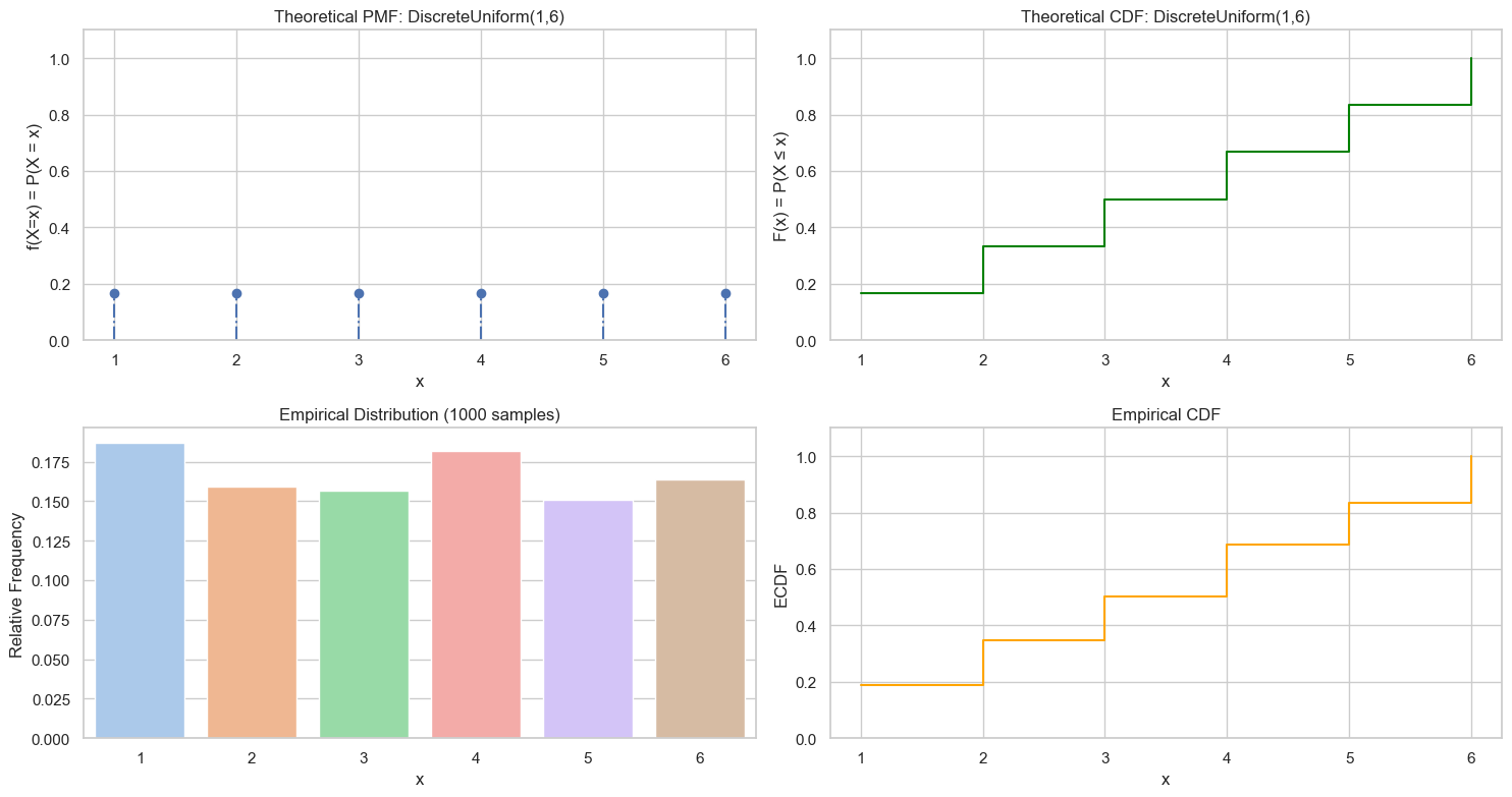
Discrete Uniform Random Variable

If a random variable $X$ takes values in a finite set of discrete numbers, and each value has the same probability of occurring, then it is a discrete uniform random variable.

Examples:

Rolling a die: $X \in \{1, 2, 3, 4, 5, 6\}$, each outcome has probability $\frac{1}{6}$
Randomly selecting a card (from 1 to 52)

Mathematical Definition

Let $X \sim \text{DiscreteUniform}(a, b)$, where $a$, $b \in \mathbb{Z}$, and $a \leq b$.

Support (Range):
$$ k \in \{a, a+1, a+2, \dots, b\} $$
Probability of each value:
$$ P(X = k) = \frac{1}{b - a + 1}, \quad \text{for } k \in \{a, \dots, b\} $$
Probability Mass Function (PMF):
$$ f(X=k) = P(X=k) = \left\{ \begin{aligned} \frac{1}{b-a+1}, \text{for } a \le k \le b\\ 0, \text{ otherwise} \end{aligned} \right. $$
Cumulative Distribution Function (CDF):
$$ F(X=k) = P(X\le k) = \left\{ \begin{aligned} 0, \text{for } k \lt a \\ \frac{k-a+1}{b-a+1}, \text{for } a \le k \le b\\ 1, \text{ for } k \gt b \end{aligned} \right. $$
Expectation ($\mu$): $\frac{a+b}{2}$
Variance ($\sigma^2$): $\frac{(b-a+1)^2-1}{12}$

import numpy as np

# Set random seed
np.random.seed(42)

# 1. Define Parameters
a, b = 1, 6  # Range
values = np.arange(a, b+1)  # Discrete values: 1~6
n = len(values)
pmf = np.ones(n) / n  # Equal probability
cdf = np.cumsum(pmf)  # CDF

# 2. Sampling
n_samples = 1000
samples = np.random.choice(values, size=n_samples, p=pmf)

# 3. Visualization
plot_discrete_rv(values, pmf, cdf, samples, f"DiscreteUniform({a},{b})")

png

Sampling

We use a Continuous Uniform Distribution $U \sim \text{Uniform}(0, 1)$ to generate discrete uniform random numbers.

Steps:

Let the interval be integers from $a$ to $b$ (inclusive), total $N = b - a + 1$ numbers.
Generate a random number $U \sim \text{Uniform}(0, 1)$.
Map $U$ to the integer range: $$ X = a + \left\lfloor U \cdot N \right\rfloor $$ ✅ The resulting integer is one of $\{a, a+1, ..., b\}$, with equal probability.

If $a=0, b=1$, then:

$N = b - a + 1 = 1 - 0 + 1 = 2$
$U \sim \text{Uniform}(0, 1)$
$X = a + \left\lfloor U \cdot N \right\rfloor = 0 + \left\lfloor U \cdot 2 \right\rfloor = \left\lfloor U \cdot 2 \right\rfloor$

Summary:

Step	Description
Goal	Sample from $\{a, a+1, ..., b\}$ with equal probability
Method	Generate $U \sim \text{Uniform}(0,1)$, then $X = a + \lfloor U \cdot (b - a + 1) \rfloor$
Function	`random.random()` or `random.randint(a, b)`
Application	Dice simulation, roulette, lottery, uniform integer sampling, etc.

import random

def discrete_uniform_sample(a, b, n):
    N = b - a + 1
    # U ~ Uniform(0, 1)
    U = [random.random() for _ in range(n)] # random.random() returns float in [0.0, 1.0)
    # X ~ Discrete Uniform(a, b)
    X = [a+int(u*N) for u in U]
    return U, X

discrete_uniform_sample(0, 1, 10)

([0.4444854289944321, 0.951251619861675, ...],
 [0, 1, 1, 1, 0, 1, 1, 1, 0, 1])

Simpler Way (Built-in)

Of course, Python provides a direct method: random.randint(a, b) # includes a and b. It implements the principle above.

[random.randint(0, 1) for _ in range(10)]  # Using built-in function to verify

[0, 1, 1, 0, 0, 1, 0, 0, 0, 0]

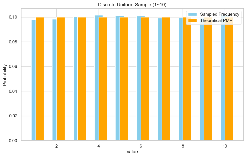
Verify Sampling Results

We sample 10,000 times to see if the distribution is uniform. You should see bar heights roughly equal for 1 to 6.

import random
import matplotlib.pyplot as plt
from math import comb

# Sampling
a, b, N = 1, 10, 30000
origin_samples, samples = discrete_uniform_sample(a, b, N)
print(f"Empirical mean: {sum(samples)/len(samples):.3f}")
# Frequency Stats
counts = [samples.count(k) / N for k in range(a, b+1)]

# Calculate Theoretical PMF
theoretical = [1/(b-a+1) for _ in range(a, b+1)]
print(f"PMF = {theoretical}")

# Step 5: Visualization
plt.figure(figsize=(10, 6))
plt.bar(range(a, b+1), counts, width=0.4, label='Sampled Frequency', color='skyblue', align='center')
plt.bar(range(a, b+1), theoretical, width=0.4, label='Theoretical PMF', color='orange', align='edge')
plt.xlabel("Value")
plt.ylabel("Probability")
plt.title(f"Discrete Uniform Sample ({a}~{b})")
plt.legend()
plt.grid(True)
plt.show()

Empirical mean: 5.515
PMF = [0.1, 0.1, 0.1, 0.1, 0.1, 0.1, 0.1, 0.1, 0.1, 0.1]

png

Continuous Uniform Random Variable

What is a Continuous Uniform Distribution?

A random variable $X \sim \text{Uniform}(a, b)$, if every value in the interval $[a, b]$ is equally likely to occur, is said to follow a continuous uniform distribution.

Mathematical Definition

Support: $X \in [a, b]$
Probability Density Function (PDF): $$ f_X(x) = \begin{cases} \frac{1}{b - a} & \text{if } x \in [a, b] \\ 0 & \text{otherwise} \end{cases} $$
Cumulative Distribution Function (CDF): $$ F_X(x) = \begin{cases} 0 & \text{if } x < a \\ \frac{x - a}{b - a} & \text{if } a \leq x \leq b \\ 1 & \text{if } x > b \end{cases} $$
Expectation ($\mu$): $\frac{a+b}{2}$
Variance ($\sigma^2$): $\frac{(b-a)^2}{12}$

Reference:

Wiki: Continuous uniform distribution

Sampling

Sampling Principle (Inverse Transform Sampling)

The simplest method is:

If $U \sim \text{Uniform}(0,1)$, then
$$ > X = a + (b - a) \cdot U \sim \text{Uniform}(a, b) > $$

💡Why?

$U \in [0, 1]$ is standard uniform.
Scaling length by $(b - a)$ and adding $a$ is a “linear map”.
Transformed $X$ is uniformly distributed on $[a, b]$.

Steps:

Step 1: Generate U ~ Uniform(0, 1)
Step 2: Linear Transform X = a + (b - a) * U
Step 3: X is your sample from Uniform(a, b)

Summary Table

Item	Content
Name	Continuous Uniform(a, b)
PDF	$f(x) = \frac{1}{b - a}$
Method	$X = a + (b - a) \cdot U$, where $U \sim \text{Uniform}(0,1)$
Python	`random.random()` or `random.uniform(a, b)`
Use Case	Monte Carlo, Simulation, Initialization

import random

def sample_uniform(a, b):
    U = random.random()        # U ~ Uniform(0,1)
    X = a + (b - a) * U        # X ~ Uniform(a, b)
    return X


def sample_uniform_list(a, b, n):
    return [sample_uniform(a, b) for _ in range(n)]

sample_uniform_list(0, 1, 10)

[0.640..., 0.059..., ...]

Directly using `uniform(a, b)`

This is the standard library wrapper, basically implementing a + (b - a) * random.random().

random.uniform(0, 1)

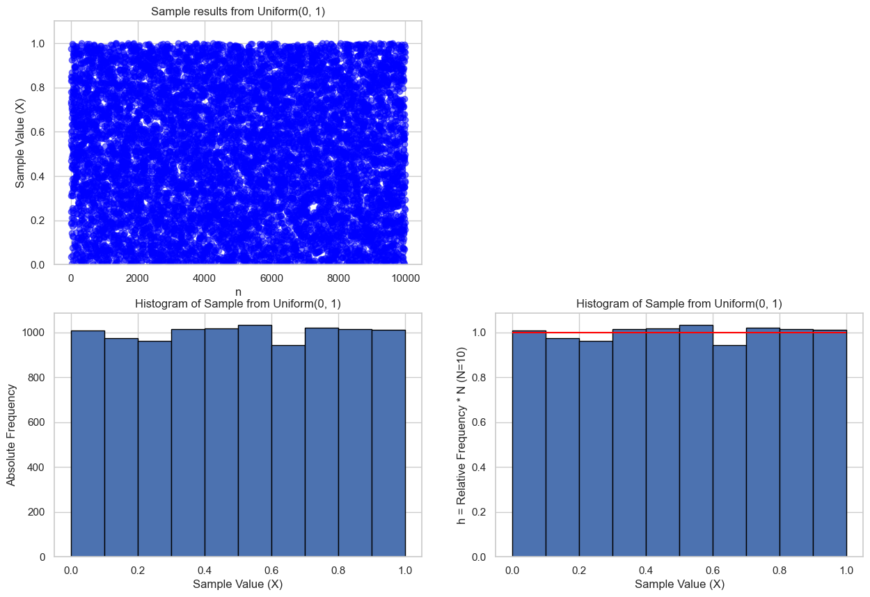
Verify Sampling Effect

Principle: Check if histogram matches the model. Sample 10,000 points from $X \sim \text{Uniform}(2, 5)$, plot histogram. ✅ If flat, it works.

import matplotlib.pyplot as plt

a, b, n = 0, 1, 10000
pdf = 1 / (b - a)  # PDF of uniform
samples = sample_uniform_list(a, b, n)

plt.figure(figsize=(15, 10))
# Sample results
plt.subplot(2, 2, 1)
plt.scatter(range(n), samples, alpha=0.5, color='blue')
plt.title(f"Sample results from Uniform({a}, {b})")
plt.xlabel("n")
plt.ylabel("Sample Value (X)")
plt.ylim(0, 1.1)

# Histogram (Frequency)
N = 10
plt.subplot(2, 2, 3)
plt.hist(samples, bins=N, density=False, edgecolor='black')
plt.title(f"Histogram of Sample from Uniform({a}, {b})")
plt.xlabel("Sample Value (X)")
plt.ylabel("Absolute Frequency")

# Histogram (Relative Frequency)
plt.subplot(2, 2, 4)
plt.hist(samples, bins=N, density=True, edgecolor='black')
plt.hlines(pdf, a, b, colors='red', linestyles='solid', label='PDF')
plt.title(f"Histogram of Sample from Uniform({a}, {b})")
plt.xlabel("Sample Value (X)")
plt.ylabel(f"h = Relative Frequency * N (N={N})")

plt.show()

png

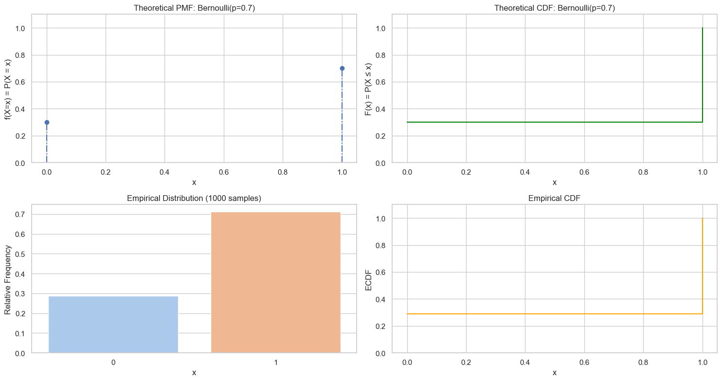
Bernoulli Random Variable

Also known as 0-1 distribution. Discrete RV.

Mathematical Definition

Let $X \sim \text{Bernoulli}(p)$, where $0 \le p \le 1$.

Support: $k \in \{0, 1\}$
Probability: $$ P(X = 1) = p \\ P(X = 0) = 1 - p $$
PMF: $$ f(X=k) = \left\{ \begin{aligned} p, \text{if } k=1\\ 1-p, \text{if } k=0 \end{aligned} \right. $$
CDF: $$ F(X=k) = \left\{ \begin{aligned} 0, \text{if } k \lt 0 \\ 1-p, \text{if } 0 \le k \lt 1\\ 1, \text{ for } k \ge 1 \end{aligned} \right. $$
Expectation ($\mu$): $p$
Variance ($\sigma^2$): $p(1-p)$

Reference: Bernoulli distribution

import numpy as np

# Set random seed
np.random.seed(42)

# 1. Define parameters
p = 0.7
values = np.array([0, 1])
n = len(values)
pmf = np.array([1-p, p])
cdf = np.cumsum(pmf)

# 2. Sampling
n_samples = 1000
samples = np.array([np.random.binomial(n=1, p=p) for _ in range(n_samples)])

# 3. Visualization
plot_discrete_rv(values, pmf, cdf, samples, f"Bernoulli(p={p})")

png

Bernoulli Theorem

Describes relationship between probability and frequency. As trials increase, relative frequency converges to probability $p$.

$$ \bar{X}_n = \frac{1}{n} \sum_{i=1}^n X_i $$$$ \lim_{n \to \infty} \mathbb{P}\left( \left| \bar{X}_n - p \right| > \epsilon \right) = 0 $$

import numpy as np
import matplotlib.pyplot as plt
from matplotlib.animation import FuncAnimation
from IPython.display import HTML

# -----------------------------
# Parameter Setting
# -----------------------------
p = 0.3                # Probability of success
n_trials = 10000       # Total trials
interval = 50          # Animation interval (ms)

# -----------------------------
# Generate Bernoulli Data
# -----------------------------
np.random.seed(0)
samples = np.random.binomial(n=1, p=p, size=n_trials)
cumulative_freq = np.cumsum(samples) / np.arange(1, n_trials + 1)

# -----------------------------
# Create Plot
# -----------------------------
fig, ax = plt.subplots(figsize=(8, 4))
ax.set_ylim(0, 1)
ax.set_xlim(1, n_trials)
ax.axhline(y=p, color='red', linestyle='--', label=f'True Probability p = {p}')
line, = ax.plot([], [], lw=2, label='Empirical Frequency')
text = ax.text(0.05, 0.9, '', transform=ax.transAxes)
ax.set_xlabel('Number of Trials')
ax.set_ylabel('Success Frequency')
ax.set_title('Bernoulli Theorem Animation')
ax.legend()

# -----------------------------
# Update Function
# -----------------------------
def update(frame):
    x = np.arange(1, frame + 1)
    y = cumulative_freq[:frame]
    line.set_data(x, y)
    text.set_text(f'n = {frame}, freq = {y[-1]:.3f}')
    return line, text

# -----------------------------
# Create Animation
# -----------------------------
ani = FuncAnimation(fig, update, frames=np.arange(1, n_trials + 1, 10),
                    interval=interval, blit=True)
# Save as GIF
from matplotlib.animation import PillowWriter
ani.save("bernoulli_theorem_animation.gif", writer=PillowWriter(fps=10))

plt.close(fig)

from IPython.display import Image
Image(filename="bernoulli_theorem_animation.gif")

png

Sampling

Based on Uniform(0, 1)

🌱 Principle Using $U \sim \text{Uniform}(0,1)$:

If $U < p$, output 1 (Success)
Else output 0 (Failure)

import matplotlib.pyplot as plt
import matplotlib.animation as animation
import numpy as np
from IPython.display import HTML

# Parameters
p = 0.3
n_frames = 100

# Pre-generate uniform samples
uniform_samples = np.random.uniform(0, 1, n_frames)
bernoulli_samples = (uniform_samples < p).astype(int)

# Set up the figure and axes
fig, axs = plt.subplots(1, 2, figsize=(12, 4))
uniform_ax = axs[0]
bernoulli_ax = axs[1]

# Initialize plots
uniform_scatter = uniform_ax.scatter([], [], c='blue', alpha=0.6)
bernoulli_bar = bernoulli_ax.bar([0, 1], [0, 0], color='orange', edgecolor='black')

# Configure uniform axis
uniform_ax.axvline(p, color='red', linestyle='--', label=f'p = {p}')
uniform_ax.set_xlim(0, 1)
uniform_ax.set_ylim(0, 1)
uniform_ax.set_title('Sampling from Uniform(0,1)')
uniform_ax.set_xlabel('Value')
uniform_ax.set_ylabel('Random Height')
uniform_ax.legend()
uniform_ax.grid(True)

# Configure Bernoulli axis
bernoulli_ax.set_xlim(-0.5, 1.5)
bernoulli_ax.set_ylim(0, n_frames)
bernoulli_ax.set_title('Bernoulli Sample Counts')
bernoulli_ax.set_xlabel('Value')
bernoulli_ax.set_ylabel('Count')
bernoulli_ax.set_xticks([0, 1])
bernoulli_ax.grid(True)

# Store sample counts
count_0 = 0
count_1 = 0
x_vals = []
y_vals = []

# Animation update function
def update(frame):
    global count_0, count_1, x_vals, y_vals

    u = uniform_samples[frame]
    x_vals.append(u)
    y_vals.append(np.random.rand())  # random y position for scatter

    bern_sample = bernoulli_samples[frame]
    if bern_sample == 0:
        count_0 += 1
    else:
        count_1 += 1

    # Update scatter
    uniform_scatter.set_offsets(np.column_stack((x_vals, y_vals)))

    # Update bar chart
    bernoulli_bar[0].set_height(count_0)
    bernoulli_bar[1].set_height(count_1)

    return uniform_scatter, bernoulli_bar

# Create animation
ani = animation.FuncAnimation(fig, update, frames=n_frames, interval=100, blit=False)
# Save as GIF
from matplotlib.animation import PillowWriter
ani.save("sample_uniform_to_bernoulli.gif", writer=PillowWriter(fps=10))

plt.close(fig)

from IPython.display import Image
Image(filename="sample_uniform_to_bernoulli.gif")

png

import random
def sample_bernoulli(p):
    U = random.random()
    return 1 if U < p else 0

p, N = 0.7, 10000
samples = [sample_bernoulli(p) for _ in range(N)]
print(f"Empirical mean: {sum(samples)/len(samples):.3f}")  # Should be close to 0.7

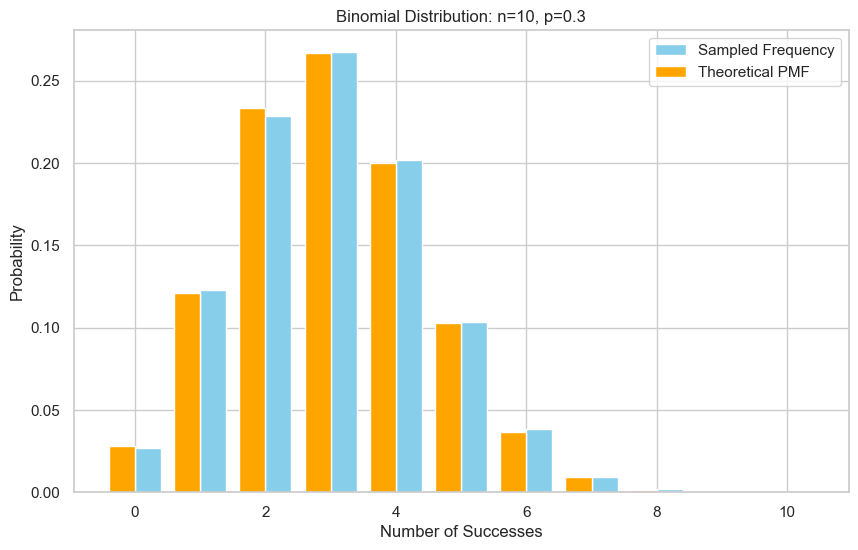
Binomial Random Variable

$X \sim \text{Binomial}(n, p)$ represents the total number of successes in $n$ independent Bernoulli trials (probability $p$).

Mathematical Definition

Support: $k \in \{0, \dots, n\}$
Probability: $$ P(X = k) = \begin{pmatrix} n \\ k \end{pmatrix}p^k(1-p)^{(n-k)} $$
Expectation: $np$
Variance: $np(1-p)$

Reference: Binomial distribution

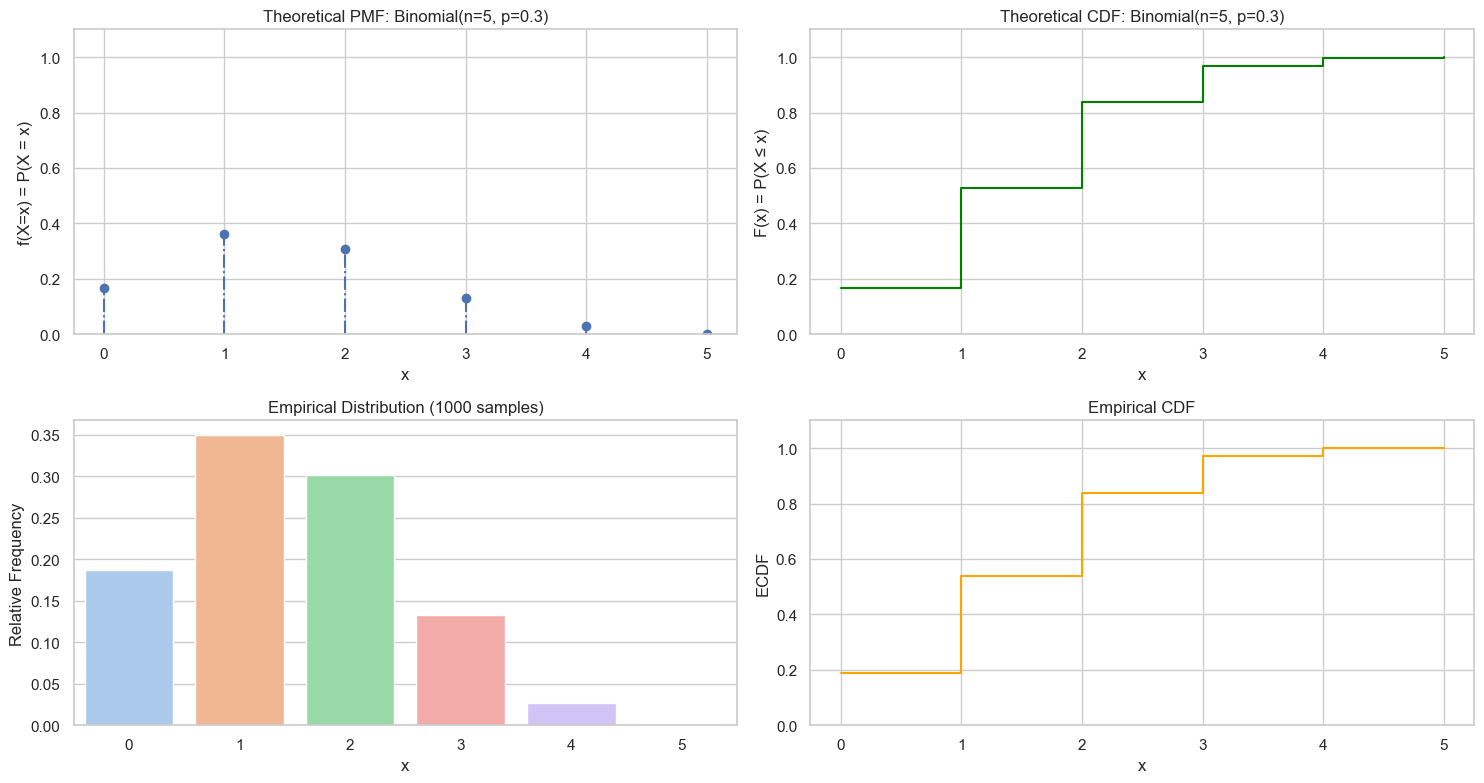
from scipy.stats import binom
import numpy as np

# Random Seed
np.random.seed(42)

# 1. Define Parameters
n, p = 5, 0.3
values = range(n + 1)
pmf = binom.pmf(values, n, p)
cdf = np.cumsum(pmf)

# 2. Sampling
n_samples = 1000
samples = np.random.binomial(n=n, p=p, size=n_samples)

# 3. Visualization
plot_discrete_rv(values, pmf, cdf, samples, f'Binomial(n={n}, p={p})')

png

Sampling Methods

Method	Idea	Scope	Exact?	Easy?
1. Repeated Bernoulli	Sum $n$ Bernoullis	Any $n, p$, especially small $n$	✅	✅
2. Inverse Transform	Find first $k$ where $F(k) \ge u$	Small $n$	✅	⚠️
3. Table Lookup	Precompute $F(k)$	Small $n$, repeated sampling	✅	✅
4. Rejection Sampling	Accept/Reject with proposal	Medium $n$, simulation	✅	⚠️
5. Normal Approx	$\mathcal{N}(np, np(1-p))$	Large $n$, $np(1-p) \ge 10$	❌	✅
6. Poisson Approx	$\text{Poisson}(np)$	Large $n$, small $p$	❌	✅
7. BTPE (NumPy)	Fast specialized algo	Any	✅	⚠️

Method 1: Repeated Bernoulli

Simple sum of $n$ coin flips.

import random

def sample_binomial_mimic(n, p):
    count = 0
    for _ in range(n): # repeat N times Bernouli sampling
        u = random.random()
        if 1-p <= u < 1:
            count += 1
    return count

def sample_binomial_mimic_list(n, p, num_samples):
    return [sample_binomial_mimic(n, p) for _ in range(num_samples)]

png

Method 2: Inverse Transform

Find $k$ such that $F(k-1) < U \le F(k)$.

import random
from math import comb

def sample_binomial_inverse(n, p):
    u = random.random()
    cumulative = 0.0
    for k in range(n + 1):
        prob = comb(n, k) * (p ** k) * ((1 - p) ** (n - k))
        cumulative += prob
        if u <= cumulative:
            return k
    return n

def sample_binomial_inverse_list(n, p, num_samples):
    return [sample_binomial_inverse(n, p) for _ in range(num_samples)]

png

Method 3: Table Lookup

Precompute CDF table for faster repeated sampling.

Method 4: Rejection Sampling

Use a proposal $g(k)$ (e.g. Uniform) and scaling $M$. png

Method 5: Normal Approximation

Use $X \approx \mathcal{N}(np, np(1-p))$. Round result to integer. Condition: $np \ge 10$ and $n(1-p) \ge 10$. Continuity correction: $X \approx \text{round}(Y + 0.5)$.

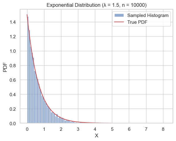
Exponential Random Variable

Continuous RV. Models time between events.

Mathematical Definition $X \sim \text{Exp}(\lambda)$.

PDF: $f(x) = \lambda e^{-\lambda x}, x \ge 0$.
CDF: $F(x) = 1 - e^{-\lambda x}, x \ge 0$.
Mean: $1/\lambda$. Variance: $1/\lambda^2$.

png

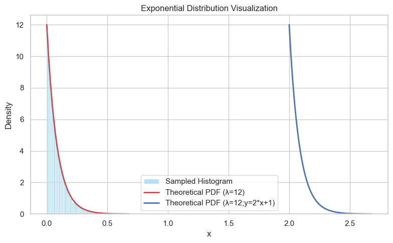
Sampling (Inverse Transform)

Formula:

$$ X = -\frac{\ln(1-U)}{\lambda} $$

Since $1-U \sim U$, simplified to $X = -\ln(U)/\lambda$.

import random
import math

def sample_exponential_inverse(lambda_val):
    u = random.random()
    return -math.log(1-u) / lambda_val

png

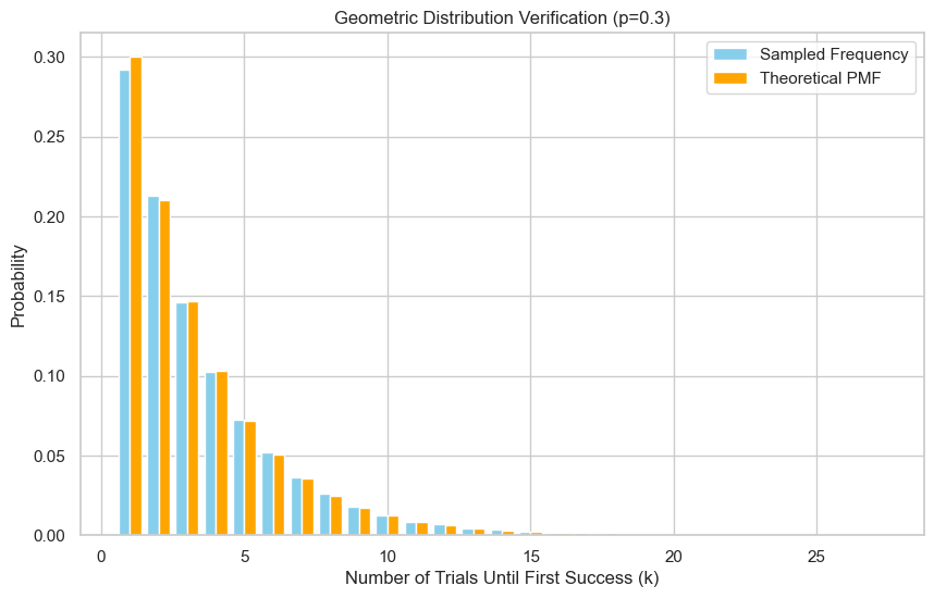
Geometric Random Variable

Discrete RV. Number of trials until first success.

Mathematical Definition $X \sim \text{Geometric}(p)$. Support $\{1, 2, \dots\}$.

PMF: $P(X=k) = (1-p)^{k-1}p$.
CDF: $P(X \le k) = 1 - (1-p)^k$.
Mean: $1/p$. Variance: $(1-p)/p^2$.

png

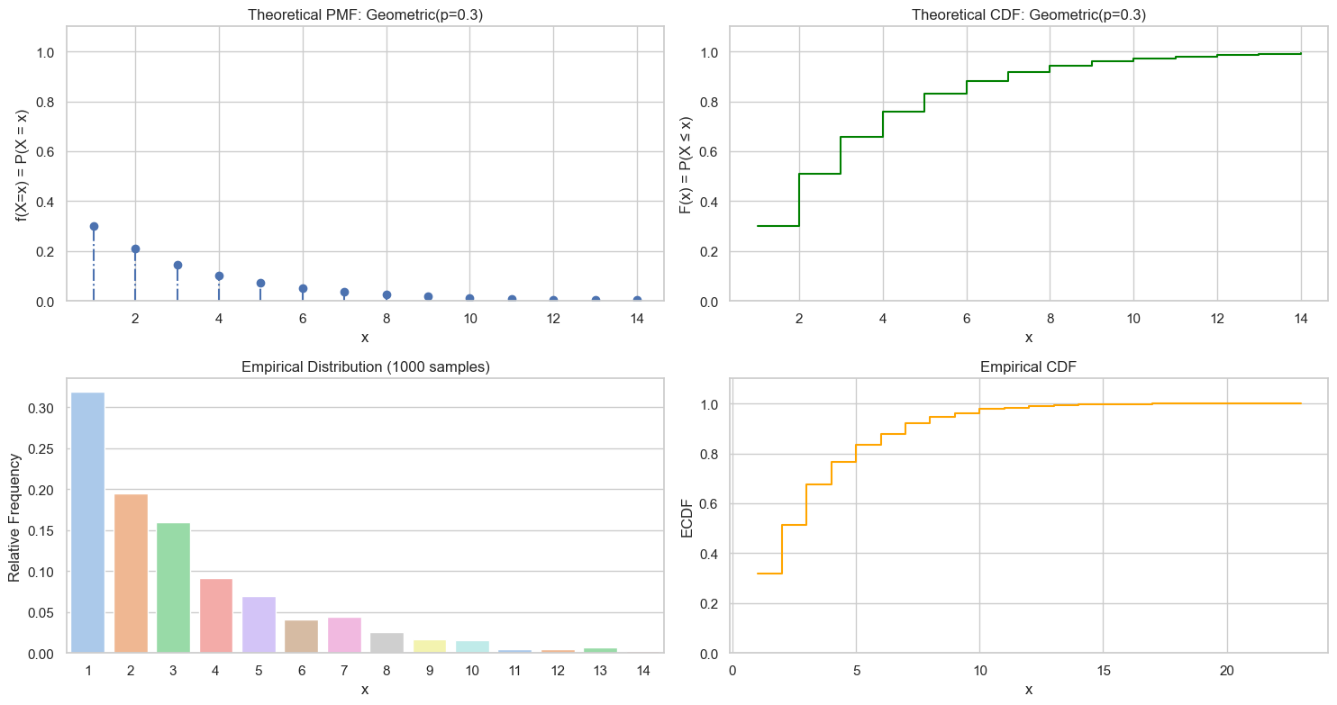
Sampling

Inverse Transform (Closed Form)

$$ k = \left\lceil \frac{\ln(1-U)}{\ln(1-p)} \right\rceil $$

Efficient ($O(1)$).

def sample_geometric_inverse(p):
    u = np.random.uniform(0, 1)
    return int(np.ceil(np.log(1 - u) / np.log(1 - p)))

png

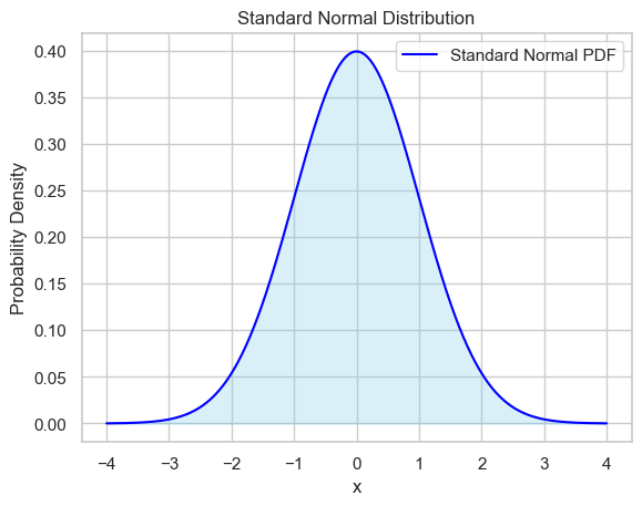
Normal Random Variable

Gaussian distribution. $f(x) = \frac{1}{\sqrt{2\pi\sigma^2}}e^{-\frac{(x-\mu)^2}{2\sigma^2}}$. Standard Normal: $\mu=0, \sigma=1$.

png

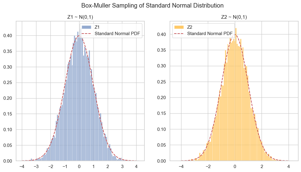
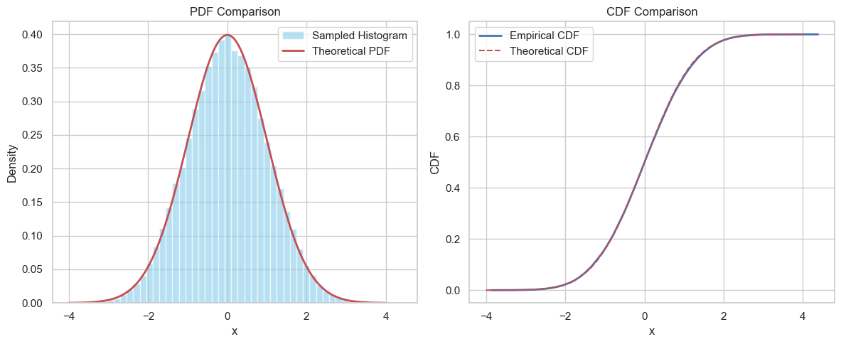
Sampling Standard Normal

Method	Principle	Note
Box-Muller	Polar transform	Exact, 2 samples at once
CLT	Sum of Uniforms	Approximate
Rejection	Envelope	General but maybe inefficient

Method 1: Box-Muller

Use two $U_1, U_2$:

$$ Z_1 = \sqrt{-2\ln U_1}\cos(2\pi U_2) \\ Z_2 = \sqrt{-2\ln U_1}\sin(2\pi U_2) $$

Both are independent $\mathcal{N}(0,1)$.

png

Method 2: CLT

Sum of 12 Uniforms: $Z = \sum_{i=1}^{12} (U_i - 0.5)$. Variance is 1.

png

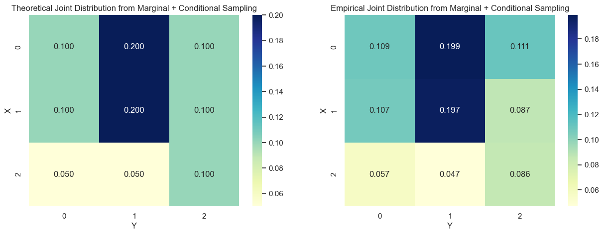
Sampling from Joint Distributions

2D Discrete

Flattening: Treat $(x,y)$ pairs as 1D list, use Inverse Transform.
Marginal + Conditional: Calculate $P(X)$, sample $x$. Calculate $P(Y|x)$, sample $y$.

png

Continuous

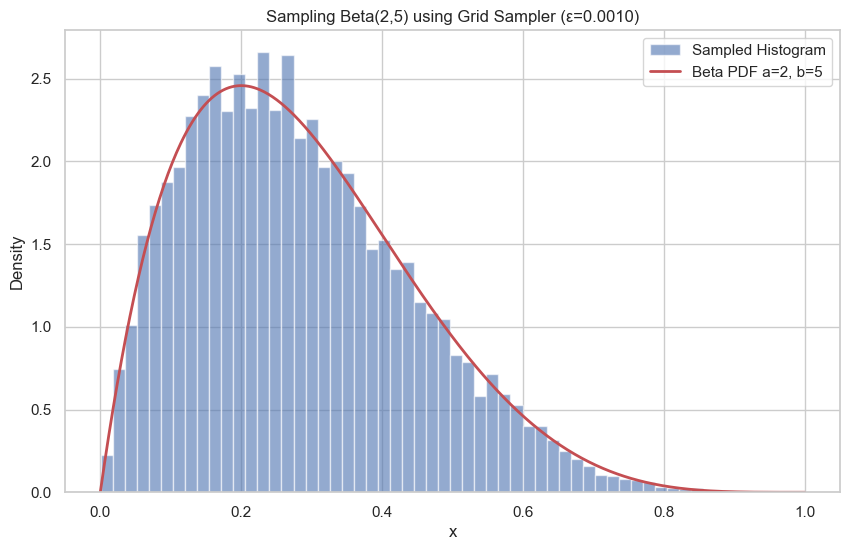
Grid Sampler

Recursively divide interval (binary tree), sample based on interval mass. Used for high-precision or when Inverse CDF is unknown but CDF is calculable.

png

Rejection Sampling (General)

Accept if $u \le \frac{f(x)}{M q(x)}$. png

Computations with Random Variables

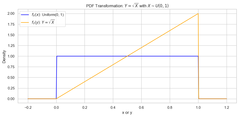
Transformation

Linear: $Y=aX+b \Rightarrow f_Y(y) = f_X(\frac{y-b}{a})|\frac{1}{a}|$. Nonlinear: $Y=g(X) \Rightarrow f_Y(y) = f_X(g^{-1}(y)) |\frac{d}{dy}g^{-1}(y)|$.

Example: $Y=\sqrt{X}, X \sim U(0,1) \Rightarrow f_Y(y) = 2y$ on $[0,1]$. png

Mean Operator ($\mathbb{E}$)

Linear operator. $\mathbb{E}[g(X)] = \int g(x)f(x)dx$.

Propagation of Error

Approximate variance of $Y=g(X)$ via Taylor expansion:

$$ \text{Var}(Y) \approx [g'(\mu_X)]^2 \text{Var}(X) $$

Multivariate:

$$ \text{Var}(Y) \approx \nabla g^T \Sigma \nabla g $$

Appendix: Sampling from Polar Coordinates

Transform known $(X,Y)$ to $(R^2, \alpha)$ via Jacobian $|J|=1/2$.

$$f_{R^2, \alpha}(u, v) = 2 f_{X,Y}(\sqrt{u} \cos v, \sqrt{u} \sin v)$$

png

Random Variables

Uniform Distribution (Uniform RV)

Discrete Uniform Random Variable

Sampling

Simpler Way (Built-in)

Verify Sampling Results

Continuous Uniform Random Variable

Sampling

Directly using uniform(a, b)

Verify Sampling Effect

Bernoulli Random Variable

Bernoulli Theorem

Sampling

Based on Uniform(0, 1)

Binomial Random Variable

Sampling Methods

Method 1: Repeated Bernoulli

Method 2: Inverse Transform

Method 3: Table Lookup

Method 4: Rejection Sampling

Method 5: Normal Approximation

Exponential Random Variable

Sampling (Inverse Transform)

Geometric Random Variable

Sampling

Inverse Transform (Closed Form)

Normal Random Variable

Sampling Standard Normal

Method 1: Box-Muller

Method 2: CLT

Sampling from Joint Distributions

2D Discrete

Continuous

Grid Sampler

Rejection Sampling (General)

Computations with Random Variables

Transformation

Mean Operator ($\mathbb{E}$)

Propagation of Error

Appendix: Sampling from Polar Coordinates

Scan to Share微信扫一扫分享

See also

目录

Directly using `uniform(a, b)`

Scan to Share
微信扫一扫分享