Three Interpretations of Probability
🔵 1. Frequentist Interpretation
🌱 Core Idea:
Probability is the limit of long-term frequency. It refers to the proportion of times an event occurs in infinitely repeated independent experiments.
Probability is the frequency of an event occurring in long-term repetitions.
📌 Mathematical Expression:
If we independently repeat an experiment $n$ times, and event $A$ occurs $n_A$ times, then:
$$ P(A) = \lim_{n \to \infty} \frac{n_A}{n} $$🧠 Key Features:
- Probability is objective and independent of the observer.
- Probability only applies to repeatable experiments (e.g., flipping coins, drawing balls, taking measurements).
- Not applicable to one-time events (e.g., predicting whether a war will happen next year).
🎯 Application Examples:
- Flipping coins, rolling dice, sample surveys
- Parameter estimation: Maximum Likelihood Estimation (MLE)
- Hypothesis testing (p-value, confidence intervals, etc.)
⚠️ Drawbacks:
- Powerless against one-time events (frequency cannot be defined)
- Cannot express subjective uncertainty (e.g., the probability of “I believe this painting is a real Picasso”)
# Re-import libraries and redraw animation code
import matplotlib.pyplot as plt
import numpy as np
import matplotlib.animation as animation

# Set random seed for reproducibility
np.random.seed(42)

# Simulate flipping a coin n times (0 for tails, 1 for heads)
n_trials = 2000
outcomes = np.random.choice([0, 1], size=n_trials)
cumulative_heads = np.cumsum(outcomes)
frequencies = cumulative_heads / np.arange(1, n_trials + 1)

# Create animation figure
fig, ax = plt.subplots()
line, = ax.plot([], [], lw=2)
ax.set_xlim(0, n_trials)
ax.set_ylim(0, 1)
ax.axhline(0.5, color='red', linestyle='--', label='True Probability = 0.5')
ax.set_xlabel('Number of Trials')
ax.set_ylabel('Frequency of Heads')
ax.set_title('Frequency Converges to Probability')
ax.legend()

def init():
    line.set_data([], [])
    return line,

def update(frame):
    x = np.arange(1, frame + 1)
    y = frequencies[:frame]
    line.set_data(x, y)
    return line,

ani = animation.FuncAnimation(fig, update, frames=np.arange(10, n_trials, 10),
                              init_func=init, blit=True)

# Save as GIF
from matplotlib.animation import PillowWriter
ani.save("frequency_converges_to_probability.gif", writer=PillowWriter(fps=10))

plt.close(fig)

from IPython.display import Image
Image(filename="frequency_converges_to_probability.gif")
# As the number of trials increases, the frequency gradually converges to the true probability (red line)
🔴 2. Bayesian Interpretation
🌱 Core Idea:
Probability is the quantification of subjective belief, used to express the observer’s “degree of belief” that an event will occur.
Probability is your subjective measure of uncertainty about an event.
📌 Mathematical Expression:
According to Bayes’ Theorem, i.e., Posterior Probability = Standardised Likelihood * Prior Probability, we have:
Where:
- $\theta$: A random variable
- $P(\theta)$:Prior (your original belief)
- $P(\text{data}|\theta)$:Likelihood (data generation mechanism)
- $P(\theta|\text{data})$:Posterior (belief updated after observing data)
- $\frac{P(\text{data}|\theta)}{P(\text{data})}$:Standardised likelihood
Deriving Bayes’ Theorem from Conditional Probability
Bayes’ Theorem can be expressed as $P(A|B) = \frac{P(A)P(B|A)}{P(B)}$. According to the definition of Conditional Probability, we have:
$$ P(A|B) = \frac{P(AB)}{P(B)} \rightarrow P(AB) = P(A|B)P(B)\\ P(B|A) = \frac{P(AB)}{P(A)} \rightarrow P(AB) = P(B|A)P(A) $$Therefore,
$$ P(A|B)P(B) = P(B|A)P(A) \rightarrow P(A|B) = \frac{P(A)P(B|A)}{P(B)} $$🧠 Key Features:
- Probability is subjective and depends on the observer’s background knowledge
- Can assign probability to any event, including one-time events
- The core mechanism is updating beliefs: prior → posterior
🎯 Application Examples:
- Medical diagnosis (doctor’s judgment on the probability of a patient being sick)
- Bayesian networks, decision systems in AI
- Parameter estimation: Bayesian inference (MCMC methods)
⚠️ Drawbacks:
- Choice of prior is subjective
- Calculation can be complex (especially when the posterior distribution is hard to resolve analytically)
import numpy as np
import matplotlib.pyplot as plt
from matplotlib.animation import FuncAnimation
from scipy.stats import beta

# Set prior parameters
a_prior, b_prior = 2, 2  # Prior ~ Beta(2,2)

# Simulate observed data (e.g., coin flipping)
np.random.seed(42)
true_p = 0.7
N_trials = 100
data = np.random.binomial(1, true_p, size=N_trials)  # 1 means heads

# Create Beta distribution animation: From prior to posterior
fig, ax = plt.subplots(figsize=(8, 5))
ax.vlines(true_p, 0, 10, colors='red', linestyles='--', label=f'True probability = {true_p}')
x = np.linspace(0.01, 0.99, 200)
line, = ax.plot([], [], lw=2)
title = ax.text(0.5, 1.05, "", ha="center", transform=ax.transAxes, fontsize=12)
ax.legend()
def init():
    ax.set_xlim(0, 1)
    ax.set_ylim(0, 10)
    ax.set_xlabel("Probability")
    ax.set_ylabel("Density")
    line.set_data([], [])
    return line, title

def update(i):
    if i == 0:
        a_post, b_post = a_prior, b_prior
    else:
        a_post = a_prior + np.sum(data[:i])
        b_post = b_prior + i - np.sum(data[:i])
    y = beta.pdf(x, a_post, b_post)
    line.set_data(x, y)
    title.set_text(f"Step {i}: Posterior ~ Beta({a_post}, {b_post})")
    return line, title

ani = FuncAnimation(fig, update, frames=N_trials + 1, init_func=init,
                    blit=True, interval=300)

# Save as GIF
from matplotlib.animation import PillowWriter
ani.save("probability_Bayesian_update_prior_to_posterior.gif", writer=PillowWriter(fps=10))

plt.close(fig)

from IPython.display import Image
Image(filename="probability_Bayesian_update_prior_to_posterior.gif")

# Core idea of Bayesianism: Our understanding of probability updates gradually with evidence, while probability itself reflects our subjective uncertainty.
⚫️ 3. Axiomatic Definition (Kolmogorov Axiomatic Approach)
🌱 Core Idea:
Probability is an abstract mathematical structure satisfying a specific axiomatic system, detached from subjective or empirical interpretations.
Probability is a mathematical measure defined on a sample space.
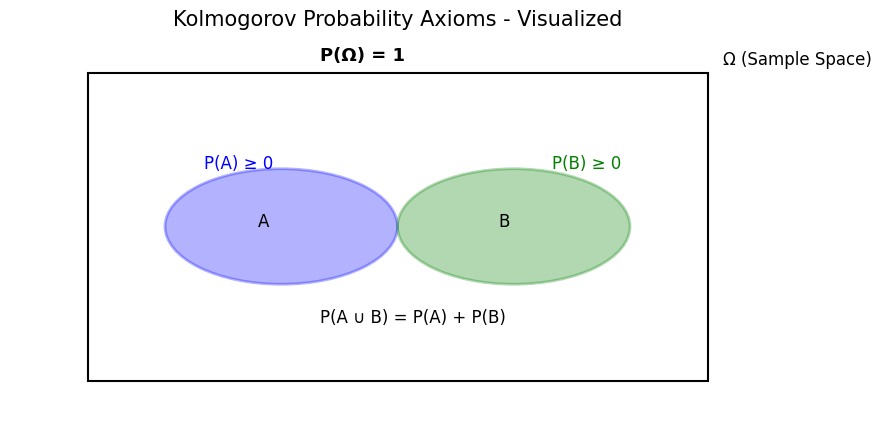
📌 Three Axioms (Kolmogorov Axioms):
Let $\Omega$ be the sample space, $\mathcal{F}$ be the set of events (σ-algebra), and $P$ be the probability function, then satisfying:
Non-negativity:
$$ \forall A \subseteq \Omega, \quad P(A) \geq 0 $$Normalization:
$$ P(\Omega) = 1 $$Countable Additivity: For any mutually exclusive events $A_1, A_2, A_3, \ldots$:
$$ P\left( \bigcup_{i=1}^{\infty} A_i \right) = \sum_{i=1}^{\infty} P(A_i) $$
Sample Space $\Omega$
A non-empty set, where elements are called outcomes or sample outputs, denoted as $\omega$.
Event Set $\mathcal{F}$
A subset of the sample space is called an event. The event set, as the name implies, is a set of events, which is a non-empty collection of subsets of the sample space $\Omega$ (subset of the power set $2^\Omega$). When we say $\mathcal{F}$ is a σ-algebra, it means $\mathcal{F}$ must satisfy the following properties:
- $\mathcal{F}$ contains the universal set, i.e., $\Omega {\in }{\mathcal {F}}$
- $A \in \mathcal{F} \rightarrow {\bar {A}} \in \mathcal{F}$
- $A_{n}{\in }{\mathcal {F}}, n=1,2,... \rightarrow \bigcup _{n=1}^{\infty }A_{n}{\in }{\mathcal {F}}$
Note: Requiring the event set to be a σ-algebra is to ensure that the results of “complement, countable union” operations are still events, so that $P$ is meaningful under these operations.
Probability Function $P:{\mathcal {F}}{\to }\mathbb {R}$
🧠 Key Features:
- Freed from frequency and subjectivity, completely built on the foundation of set theory and measure theory
- Is the foundation of modern probability theory and stochastic processes
- Compatible with both Frequentist and Bayesian interpretations
🎯 Application Examples:
- Rigorous definition of probability space, expectation, random variables
- Supporting advanced probability theory and statistics (such as Markov processes, Brownian motion)
- Abstract modeling in computer stochastic simulation
⚠️ Drawbacks:
- Does not explain “what probability actually is”, only describes “what rules probability should satisfy”
- Not intuitive enough for beginners
import matplotlib.pyplot as plt
from matplotlib_venn import venn2, venn3
import matplotlib.patches as patches

# Set up canvas
fig, ax = plt.subplots(figsize=(10, 5))

# Display a universal set Ω
omega = patches.Rectangle((0.1, 0.1), 0.8, 0.8, linewidth=1.5, edgecolor='black', facecolor='none')
ax.add_patch(omega)
ax.text(0.92, 0.92, 'Ω (Sample Space)', fontsize=12)

# Two events A and B (disjoint)
circle_A = patches.Circle((0.35, 0.5), 0.15, linewidth=2, edgecolor='blue', facecolor='blue', alpha=0.3)
circle_B = patches.Circle((0.65, 0.5), 0.15, linewidth=2, edgecolor='green', facecolor='green', alpha=0.3)

ax.add_patch(circle_A)
ax.add_patch(circle_B)
ax.text(0.32, 0.5, 'A', fontsize=12)
ax.text(0.63, 0.5, 'B', fontsize=12)

# Label probabilities
ax.text(0.25, 0.65, 'P(A) ≥ 0', fontsize=12, color='blue')
ax.text(0.7, 0.65, 'P(B) ≥ 0', fontsize=12, color='green')
ax.text(0.4, 0.25, 'P(A ∪ B) = P(A) + P(B)', fontsize=12, color='black')

# Probability of the entire space is 1
ax.text(0.4, 0.93, 'P(Ω) = 1', fontsize=13, weight='bold')

# Remove axes
ax.axis('off')
plt.title("Kolmogorov Probability Axioms - Visualized", fontsize=15)
plt.show()
📌 Summary
| Interpretation | Probability Meaning | Applicable Scenario | Representative Figure/Idea |
|---|---|---|---|
| Frequentist | Long-term frequency | Repeatable experiments | Von Mises, Fisher |
| Bayesian | Subjective belief | One-time events, cognitive decision-making | Thomas Bayes, Laplace |
| Axiomatic | Abstract measure | Theoretical modeling, rigorous mathematical derivation | Andrey Kolmogorov |
- Frequentist Interpretation: Probability is the frequency in long-term experiments → Objective empiricism.
- Bayesian Interpretation: Probability is the quantification of subjective belief → Belief update mechanism.
- Axiomatic Definition: Probability is a mathematical function satisfying certain rules → Abstract structuralism.
Events and Sample Space
Sample Space
(Intuitive) Definition: The sample space, denoted as $\Omega$, is the set of all possible outcomes of a random experiment.
Discrete Sample Space: Outcomes are countable (or finite). For example, rolling a six-sided die:
$$ \Omega=\{1,2,3,4,5,6\}. $$Or flipping a coin three times, total $2^3=8$ possible sequences: $\{HHH, HHT,\dots, TTT\}$.
Continuous Sample Space: Outcomes are intervals of continuous values or sets of real numbers, which cannot be enumerated one by one. For example, measuring someone’s height (meters):
$$ \Omega = [0, +\infty) \quad\text{or more commonly } \Omega=\mathbb{R}. $$Or considering position as a real number on $[0,1]$ (uniform distribution example).
Key Point: The sample space is where “we list all possible basic situations”. Discrete can be counted, continuous cannot be counted.
Event
(Intuitive) Definition: An event is a subset of the sample space — a set of all sample points “satisfying a certain condition”. An event can contain one outcome (atomic event) or many outcomes.
Common Event Types:
- Elementary event: Contains only one outcome. E.g., getting a 3 when rolling a die: $\{3\}$.
- Compound event: Contains multiple outcomes, e.g., “rolling an even number” $= \{2,4,6\}$.
- Certain event: Equals the entire sample space $\Omega$ (probability is 1).
- Impossible / null event: Empty set $\varnothing$ (probability is 0).
Operations on Events
Given events $A, B$, we can perform:
- Union ($A\cup B$: A or B happens)
- Intersection ($A\cap B$: Both happen)
- Complement ($A^c$: A does not happen)
Example (Rolling a Die):
- $A$: “Rolling an even number” $=\{2,4,6\}$.
- $B$: “Rolling > 3” $=\{4,5,6\}$.
- Then $A\cap B=\{4,6\}$, $A\cup B=\{2,4,5,6\}$.
How to Assign “Probability” to Events
For Discrete: Assign a probability $P(\{\omega\})$ to each elementary outcome $\omega \in \Omega$, satisfying that their sum is 1. The probability of event $A$ is the sum of probabilities of the basic outcomes it contains:
$$ P(A)=\sum_{\omega\in A}P(\{\omega\}). $$For Continuous: Cannot directly assign probability to a single point (usually 0), but use Probability Density Function (PDF) $f(x)$. The probability of event $A$ is the integral over $A$:
$$ P(A)=\int_A f(x)\,dx. $$
Three Common Examples
A. Rolling a Die (Discrete, Simple)
- Sample space $\Omega=\{1,2,3,4,5,6\}$ (if uniform, each face prob 1/6).
- Event: $A=\{\text{even}\}=\{2,4,6\}$
- Then probability of event $A$ is: $P(A)=3\times\frac{1}{6}=\frac{1}{2}$.
B. Weather Forecast (Finite Discrete, but Probabilistic)
- Sample space could be $\Omega=\{\text{Sunny},\text{Cloudy},\text{Rainy}\}$.
- Based on history we might estimate $P(\text{Sunny})=0.6,\ P(\text{Cloudy})=0.3,\ P(\text{Rainy})=0.1$.
- Event: Tomorrow “Not Rainy” $= \{\text{Sunny},\text{Cloudy}\}$, probability $0.9$.
Note: The weather example shows cases where “probability is estimated based on historical frequency or models” (interpreted by either frequency or Bayesian).
C. Image Classification (High-dimensional, Uncountable Discrete)
- Abstractly: Sample space is “set of all possible digital images”, denoted as $ \Omega = \{\text{all } H\times W\times 3 \text{ pixel matrices}\}$.
- Event e.g., “image contains a cat” is $A\subset\Omega$: set of all images labeled as cat. You cannot enumerate or assign point-wise, but can approximate $P(A)$ using models (classifiers) or datasets.
- This shows: Events don’t have to be “enumerable sets”, they can be very large sets (requiring probabilistic models, density estimation, or empirical frequencies to handle).
Basic Properties of Probability
Basic corollaries derived from Kolmogorov axioms
Proposition 1: Probability of empty event is 0
$\displaystyle P(\varnothing)=0.$
Proof: Since $\Omega$ and empty set are complementary and $\Omega=\varnothing\cup\Omega$, by Countable Additivity (taking sequence $A_1=\Omega,A_2=\varnothing,A_3=\varnothing,\dots$), or more simply noting $\Omega$ and $\varnothing$ are disjoint and $P(\Omega)=1$. A more standard proof method uses additivity:
$$ P(\Omega)=P(\varnothing\cup\Omega)=P(\varnothing)+P(\Omega)\Rightarrow P(\varnothing)=0. $$(Unique solution obtained using Non-negativity)
Proposition 2: Monotonicity
If $A\subseteq B$ (both are events), then $P(A)\le P(B)$.
Proof: Write $B=A\cup (B\setminus A)$, and $A$ and $B\setminus A$ are disjoint. By Additivity and Non-negativity:
$$ P(B)=P(A)+P(B\setminus A)\ge P(A). $$Proposition 3: Complement Rule
$\displaystyle P(A^c)=1-P(A)$.
Proof: From $A\cup A^c=\Omega$ and $A\cap A^c=\varnothing$, applying Additivity:
$$ P(\Omega)=P(A)+P(A^c)=1\Rightarrow P(A^c)=1-P(A). $$Proposition 4: Addition Formula for Two Events (with Intersection Correction Term)
$$ P(A\cup B)=P(A)+P(B)-P(A\cap B). $$Proof (Partition Method): Divide $A$ and $B$ into three disjoint parts:
$$ A=(A\setminus B)\cup(A\cap B),\quad B=(B\setminus A)\cup(A\cap B). $$And
$$ A\cup B=(A\setminus B)\cup(A\cap B)\cup(B\setminus A) $$The three parts are pairwise disjoint, applying Additivity we get:
$$ P(A) = P(A\setminus B) + P(A\cap B) \rightarrow P(A\setminus B) = P(A) - P(A\cap B) \\ P(B) = P(B\setminus A) + P(A\cap B) \rightarrow P(B\setminus A) = P(B) - P(A\cap B) \\ P(A\cup B) =P(A\setminus B) + P(A\cap B) + (B\setminus A) = P(A) - P(A\cap B) + P(A\cap B) + P(B) - P(A\cap B) = P(A) + P(B) - P(A\cap B) $$Q.E.D.
Proposition 5: Inclusion-Exclusion Principle (Two and Three Events)
- Two events: Same as above (Addition Formula).
- Three events:
Proof: Decompose the three sets into disjoint minimal atoms (8 atoms), or derive recursively from the two-set formula and subtract multiple counts (standard inclusion-exclusion derivation).
Proposition 6: Finite Additivity (Degenerated from Countable Additivity)
If $A_1,\dots,A_n$ are pairwise disjoint, then
$$ P\Big(\bigcup_{i=1}^n A_i\Big)=\sum_{i=1}^n P(A_i). $$This is a direct special case of the axiom (just take finite terms).
Proposition 7: Upper Bound of Union (Boole’s Inequality / Union bound)
For any sequence of events (not necessarily mutually exclusive) $A_1,A_2,\dots$, we have
$$ P\Big(\bigcup_{i=1}^\infty A_i\Big)\le \sum_{i=1}^\infty P(A_i). $$Key point of proof: Split the union into disjoint subsets or directly use monotonicity and countable additivity (can write union as disjoint sequence $B_1=A_1, B_2=A_2\setminus A_1, \dots$), thereby obtaining the upper bound.
Proposition 8: Continuity (From Above and Below)
- Continuity from above: If $A_1\supseteq A_2\supseteq\cdots$ and intersection $\bigcap_n A_n=\varnothing$, then $P(A_n)\downarrow 0$ (tends to 0).
- Continuity from below: If $A_1\subseteq A_2\subseteq\cdots$ and union $\bigcup_n A_n=A$, then $P(A_n)\uparrow P(A)$.
These are standard conclusions directly given by combining countable additivity with monotonicity (detailed proofs can be found in textbooks).
Conditional Probability and Multiplication Rule
Conditional Probability $P(A\mid B)$ (Rigorous Definition)
In probability space $(\Omega,\mathcal F,P)$, if $P(B)>0$, define
$$ P(A\mid B)\;\;\stackrel{\text{def}}=\;\;\frac{P(A\cap B)}{P(B)}. $$Intuitive meaning: The relative probability of $A$ in the world where “$B$ occurred”.
Rigorous Properties (Treat $P(\cdot\mid B)$ as a “new probability measure” after fixing $B$):
Non-negativity: $P(A\mid B)\ge 0$;
Normalization: $P(\Omega\mid B)=\dfrac{P(\Omega\cap B)}{P(B)}=\dfrac{P(B)}{P(B)}=1$;
Countable Additivity: If $\{A_i\}$ are pairwise disjoint, then
$$ P\Big(\bigcup_i A_i\;\Big|\;B\Big)=\frac{P\big((\bigcup_i A_i)\cap B\big)}{P(B)} =\frac{\sum_i P(A_i\cap B)}{P(B)}=\sum_i P(A_i\mid B). $$
Therefore $P(\cdot\mid B)$ satisfies Kolmogorov axioms and is a conditional probability measure.
Note: When $P(B)=0$, the above formula fails; more general cases use “Regular Conditional Probability” (Radon–Nikodym theorem gives existence), no need to worry in discrete cases.
Joint Probability $P(A\cap B)$ and Multiplication Rule
From the definition, we immediately get the Multiplication Rule:
$$ \boxed{\,P(A\cap B)=P(A\mid B)\,P(B)\,}\qquad(P(B)>0) $$Similarly, $P(A\cap B)=P(B\mid A)\,P(A)$ (if $P(A)>0$).
Chain Rule (Multiple Events): For $A_1,\dots,A_n$, if conditional probabilities are defined,
$$ P\Big(\bigcap_{k=1}^n A_k\Big) = P(A_1)\cdot P(A_2\mid A_1)\cdot P(A_3\mid A_1\cap A_2)\cdots P(A_n\mid A_1\cap\cdots\cap A_{n-1}). $$Continuous/Discrete Variable Version: $f_{X,Y}(x,y)=f_{X\mid Y}(x\mid y)f_Y(y)$; discrete $p_{X,Y}(x,y)=p_{X\mid Y}(x\mid y)p_Y(y)$.
Examples
Example A: Drawing Cards (Without Replacement)
Standard 52 cards, let
- $A_1=\{\text{First card is A (ace)}\}$
- $A_2=\{\text{Second card is A}\}$
Goal: $P(A_1\cap A_2)$.
By multiplication rule: $P(A_1\cap A_2)=P(A_1)\cdot P(A_2\mid A_1)$.
Example B: Medical Testing (Bayes derived from Multiplication Rule)
Assume:
- Disease prevalence (Prior) $\pi=P(D)$
- Sensitivity $Se=P(T^+\mid D)$
- Specificity $Sp=P(T^-\mid \bar D)\Rightarrow P(T^+\mid \bar D)=1-Sp$
Positive Predictive Value (PPV):
$$ P(D\mid T^+)=\frac{P(T^+\mid D)P(D)}{P(T^+)} =\frac{Se\cdot \pi}{Se\cdot \pi+(1-Sp)\cdot (1-\pi)}. $$This is just substituting back via multiplication rule, and using Total Probability $P(T^+)=P(T^+\mid D)\pi+P(T^+\mid \bar D)(1-\pi)$.
Summary
- Definition: $P(A\mid B)=P(A\cap B)/P(B)$; it is a probability measure itself.
- Multiplication: $P(A\cap B)=P(A\mid B)P(B)$. Generalized to Chain Rule.
- Application: Drawing cards/without replacement, medical testing all directly use multiplication rule; Bayes formula = Multiplication Rule + Total Probability.
Law of Total Probability and Bayes’ Theorem
Law of Total Probability (LTP)
Rigorous Statement (Discrete/Countable Partition)
Let $(\Omega,\mathcal F,P)$ be a probability space, $\{B_i\}_{i\in I}\subset\mathcal F$ form a countable partition of $\Omega$ (pairwise disjoint and union is $\Omega$), and $P(B_i)>0$. For any event $A\in\mathcal F$,
$$ \boxed{P(A)=\sum_{i\in I} P(A\mid B_i)\,P(B_i).} $$Proof (By Countable Additivity + Definition of Conditional Probability)
Since $\{B_i\}$ partition $\Omega$, we have
$$ A=\bigcup_{i}(A\cap B_i),\qquad (A\cap B_i)\ \text{pairwise disjoint}. $$By Countable Additivity,
$$ P(A)=\sum_i P(A\cap B_i)=\sum_i \frac{P(A\cap B_i)}{P(B_i)}\,P(B_i)=\sum_i P(A\mid B_i)\,P(B_i). $$Continuous/Density Version (Common Equation)
If $(X,Y)$ has joint density $f_{X,Y}$, then
$$ \boxed{f_X(x)=\int f_{X\mid Y}(x\mid y)\,f_Y(y)\,dy,} $$This is the sum of conditional density weighted by marginal $f_Y$ for “all $y$”; for event $A$:
$$ P(X\in A)=\int P(X\in A\mid Y=y)\,f_Y(y)\,dy. $$(More generally, conditional probability can be given by Radon–Nikodym theorem, not expanded here.)
# Draw a probability tree diagram to show the calculation path of the Law of Total Probability
import matplotlib.pyplot as plt

# Data
labels = [
    "Disease", "Healthy",
    "Pos(Disease)", "Neg(Disease)",
    "Pos(Healthy)", "Neg(Healthy)"
]
probs = [
    p_disease, 1 - p_disease,
    p_test_pos_given_disease, 1 - p_test_pos_given_disease,
    p_test_pos_given_healthy, 1 - p_test_pos_given_healthy
]

# Simple tree drawing
fig, ax = plt.subplots(figsize=(8,5))
ax.axis("off")

# Layer 1
ax.text(0.05, 0.5, "Population", fontsize=12, ha="center")
ax.plot([0.1, 0.3], [0.5, 0.7], 'k-')
ax.plot([0.1, 0.3], [0.5, 0.3], 'k-')

# Layer 2
ax.text(0.35, 0.7, f"Disease\n({p_disease:.2f})", ha="center")
ax.text(0.35, 0.3, f"Healthy\n({1-p_disease:.2f})", ha="center")
ax.plot([0.4, 0.6], [0.7, 0.8], 'k-')
ax.plot([0.4, 0.6], [0.7, 0.6], 'k-')
ax.plot([0.4, 0.6], [0.3, 0.4], 'k-')
ax.plot([0.4, 0.6], [0.3, 0.2], 'k-')

# Layer 3
ax.text(0.65, 0.8, f"Pos\n({p_test_pos_given_disease:.2f})", ha="center")
ax.text(0.65, 0.6, f"Neg\n({1-p_test_pos_given_disease:.2f})", ha="center")
ax.text(0.65, 0.4, f"Pos\n({p_test_pos_given_healthy:.2f})", ha="center")
ax.text(0.65, 0.2, f"Neg\n({1-p_test_pos_given_healthy:.2f})", ha="center")

plt.show()
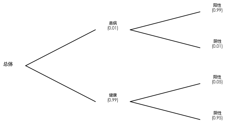
# Simulation using medical testing scenario:
# 1. Prior probability of disease is very low
# 2. Test has certain accuracy
# Code below directly reflects the idea of "partitioning population into mutually exclusive events, then summing up".
import numpy as np

# Parameters
p_disease = 0.01     # Prevalence: P(Disease)
p_test_pos_given_disease = 0.99   # P(Pos|Disease)
p_test_pos_given_healthy = 0.05   # False positive: P(Pos|Healthy)

# Total Probability Formula:
# P(Test Pos) = P(Pos|Disease)P(Disease) + P(Pos|Healthy)P(Healthy)
p_positive = (p_test_pos_given_disease * p_disease +
              p_test_pos_given_healthy * (1 - p_disease))

print(f"P(Test Pos) = {p_positive:.4f}")
P(Test Pos) = 0.0594
Bayes’ Theorem
Basic Form (Two Events)
If $P(B)>0$,
$$ \boxed{P(A\mid B)=\frac{P(B\mid A)\,P(A)}{P(B)}.} $$Directly obtained from Multiplication Rule $P(A\cap B)=P(A\mid B)P(B)=P(B\mid A)P(A)$.
Expand denominator using Total Probability (partition $\{A,\bar A\}$):
$$ P(B)=P(B\mid A)P(A)+P(B\mid \bar A)P(\bar A), $$So
$$ P(A\mid B)=\frac{P(B\mid A)P(A)} {P(B\mid A)P(A)+P(B\mid \bar A)(1-P(A))}. $$Multi-Hypothesis Version (Countable Partition $\{H_i\}$)
$$ \boxed{P(H_i\mid E)=\frac{P(E\mid H_i)\,P(H_i)}{\sum_j P(E\mid H_j)\,P(H_j)}.} $$Continuous/Density Version
$$ \boxed{f_{\Theta\mid X}(\theta\mid x)=\frac{f_{X\mid \Theta}(x\mid \theta)\,\pi(\theta)}{\int f_{X\mid \Theta}(x\mid t)\,\pi(t)\,dt}}, $$Where $\pi(\theta)$ is prior density, denominator is evidence (marginal likelihood).
The Power of “Reversing Causality” (diagnostic vs. causal)
- Likelihood $P(E\mid H)$: Causal Forward (Assume $H$ is true, how likely to see evidence $E$?)
- Posterior $P(H\mid E)$: Diagnostic Backward (Observed evidence $E$, what is the probability it was caused by $H$?)
The two are asymmetric: Large $P(E\mid H)$ does not imply large $P(H\mid E)$. Must combine with prior (base rate) and reverse using Bayes formula:
$$ \text{Posterior odds}=\text{Prior odds}\times \underbrace{\frac{P(E\mid H)}{P(E\mid \bar H)}}_{\text{Bayes Factor / Likelihood Ratio}}. $$This is why Base-rate fallacy leads to serious misjudgment.
# Using P(Test Pos) calculated in previous step, infer "Probability of really being sick given positive":
# Bayes Theorem:
# P(Disease|Pos) = [P(Pos|Disease) * P(Disease)] / P(Pos)
p_disease_given_positive = (p_test_pos_given_disease * p_disease) / p_positive

print(f"P(Disease|Pos) = {p_disease_given_positive:.4f}")
# This value is significantly smaller than intuition (because of low prior + existing false positive rate), demonstrating the power of "Reversing Causal Relation".
P(Disease|Pos) = 0.1667
Application Examples
Spam Filter (Naive Bayes Idea)
Assume $H\in\{\text{spam},\text{ham}\}$, features $E=(w_1,\dots,w_d)$ indicate presence of certain words. Naive Bayes assumes conditional independence:
$$ P(E\mid H)=\prod_{k=1}^d P(w_k\mid H). $$Posterior:
$$ P(\text{spam}\mid E)=\frac{\left(\prod_k P(w_k\mid \text{spam})\right)P(\text{spam})} {\sum_{h\in\{\text{spam},\text{ham}\}}\left(\prod_k P(w_k\mid h)\right)P(h)}. $$Intuition: Some “strong indicator words” make $P(E\mid \text{spam})$ much larger than $P(E\mid \text{ham})$, multiplied by prior $P(\text{spam})$, making posterior skew towards spam.
Mini Exercise (No calculation): If a blacklisted domain appears (feature $w$), explain why “Likelihood Ratio” $\frac{P(w\mid \text{spam})}{P(w\mid \text{ham})}$ is key to discrimination power?
Fault Diagnosis (Multi-Hypothesis Bayes)
Assume a device has three mutually exclusive faults $H_1,H_2,H_3$ and “Normal” $H_0$, prior $\{P(H_i)\}$ known. Sensor reading $E$’s distribution $P(E\mid H_i)$ known (or approximated as normal, exponential etc.). After observing $E=e$:
$$ P(H_i\mid e)=\frac{P(e\mid H_i)P(H_i)}{\sum_{j=0}^3 P(e\mid H_j)P(H_j)}. $$Intuition: Whichever $H_i$ occurs more often (large prior) AND produces current observation more likely (large likelihood), occupies larger posterior.
Summary
- Total Probability: Partition “situations”, weighted sum of “Total Prob = Cond Prob × Weight”.
- Bayes: Posterior $\propto$ Likelihood × Prior; Denominator is Total Prob of Evidence.
- Reversing Causality: Use $P(E\mid H)$ to infer $P(H\mid E)$, must multiply by prior; think in Likelihood Ratio / Odds.
Independence and Conditional Independence
Rigorous Definition and Equivalent Characterization
Event Independence
In probability space $(\Omega,\mathcal F,P)$, events $A,B\in\mathcal F$ are independent if
$$ \boxed{P(A\cap B)=P(A)\,P(B).} $$If $P(B)>0$, equivalent to
$$ P(A\mid B)=\frac{P(A\cap B)}{P(B)}=P(A). $$Indicator function characterization: Let $1_A,1_B$ be indicator functions, then independent $\iff\ \mathbb E[1_A1_B]=\mathbb E[1_A]\mathbb E[1_B]$.
Mutual Independence: $\{A_i\}_{i=1}^n$ are mutually independent if any subset intersection satisfies multiplication, e.g.
$$ P\!\Big(\bigcap_{i\in S} A_i\Big)=\prod_{i\in S}P(A_i)\quad(\forall S\subset\{1,\dots,n\},S\neq\varnothing). $$Note: “Pairwise independent” does not equal “Mutually independent”.
Different from “Disjoint”: If $A\cap B=\varnothing$ and $P(A),P(B)>0$, then $P(A\cap B)=0\ne P(A)P(B)$, so impossible to be independent.
# A simple example: Rolling two fair dice. Event A is "First die is 6", Event B is "Second die is 6".

import numpy as np

# Simulation count
N = 1_000_000

# Roll two dice
die1 = np.random.randint(1, 7, N)
die2 = np.random.randint(1, 7, N)

# Define events
A = (die1 == 6)
B = (die2 == 6)

# Calculate probabilities
P_A = A.mean()
P_B = B.mean()
P_A_and_B = (A & B).mean()

print("P(A) =", P_A)
print("P(B) =", P_B)
print("P(A ∩ B) =", P_A_and_B)
print("P(A)*P(B) =", P_A * P_B)

# Theoretically: P(A) = 1/6 = 0.1666666667, P(B) = 1/6 = 0.1666666667, P(A∩B) = 1/36 = 0.02777777778 = P(A)P(B).
# If results are close to theoretical values, A and B are independent.
P(A) = 0.16706
P(B) = 0.166036
P(A ∩ B) = 0.02781
P(A)*P(B) = 0.027737974159999994
Conditional Independence
Given σ-algebra $\mathcal G$ (or given random variable/event $C$ generating $\sigma(C)$), $A, B$ are conditionally independent given $\mathcal G$ if
$$ \boxed{\mathbb E[1_A1_B\,\mid\,\mathcal G]=\mathbb E[1_A\,\mid\,\mathcal G]\ \mathbb E[1_B\,\mid\,\mathcal G]\quad\text{a.s.}} $$Equivalently (often used in discrete case where $P(C)>0$)
$$ \boxed{P(A\cap B\mid C)=P(A\mid C)\,P(B\mid C)\quad\text{(for almost all values of }C\text{)}.} $$Important Relations:
- Conditional independence does not imply unconditional independence; Unconditional independence does not imply conditional independence.
- Common structure: Common Cause $C$ makes $A, B$ correlated; conditioning on $C$ often makes them “more independent”. Conversely, conditioning on Common Effect (collider) “introduces” correlation (Berkson’s Paradox).
# Assume a sensor light system:
#   Event A: Someone in room
#   Event B: Light on
#   Condition C: Dark outside
# Simulate: When dark, light on depends only on "someone in room", and given dark, person and light status don't affect each other (causal direction) -- Wait, actually P(B|A, C) = P(B|A) in this causal model? No, usually meant: Given C (Dark), A and B? Actually usually C causes A and B?
# Let's use the code logic:
# When C is True (Dark): A (Someone) occurs with prob 0.6, B (Light) occurs with prob 0.7 independently? No, the code says:
# A_given_C = rand < 0.6
# B_given_C = rand < 0.7
# This implies A and B are generated INDEPENDENTLY given C.

# Simulation count
N = 1_000_000

# Condition C: Dark
C = np.random.rand(N) < 0.5  # 50% prob dark

# Given dark: Someone prob 0.6, Light prob 0.7
A_given_C = np.random.rand(N) < 0.6
B_given_C = np.random.rand(N) < 0.7

# Given not dark (~C): Someone 0.3, Light 0.1
A_given_notC = np.random.rand(N) < 0.3
B_given_notC = np.random.rand(N) < 0.1

# Assign based on C
A = np.where(C, A_given_C, A_given_notC)
B = np.where(C, B_given_C, B_given_notC)

# Calculate conditional probabilities
mask_C = C  # Consider only dark cases
P_A_and_B_given_C = (A & B & mask_C).sum() / mask_C.sum() # P(A ∩ B | C) = P(A ∩ B ∩ C) / P(C)
P_A_given_C = (A & mask_C).sum() / mask_C.sum() # P(A|C)
P_B_given_C = (B & mask_C).sum() / mask_C.sum() # P(B|C)

print("P(A ∩ B | C) =", P_A_and_B_given_C)
print("P(A|C) * P(B|C) =", P_A_given_C * P_B_given_C)

# If P(A ∩ B | C) ≈ P(A|C) * P(B|C), then A and B are conditionally independent given C.
P(A ∩ B | C) = 0.420284111266571
P(A|C) * P(B|C) = 0.4200211083400713
Two Rigorous Corollaries
(i) Independence ⇒ Conditional Probability Invariant If $A\perp B$ and $P(B)>0$, then $P(A\mid B)=P(A)$.
(ii) Conditional Independence + Total Probability If given $\mathcal G$ we have $A\perp B\mid \mathcal G$, then
$$ P(A\cap B)=\mathbb E\!\big[\,P(A\cap B\mid\mathcal G)\,\big] =\mathbb E\!\big[\,P(A\mid\mathcal G)\,P(B\mid\mathcal G)\,\big]. $$Unless $P(A\mid\mathcal G)$ is constant (independent of $\mathcal G$), generally $\mathbb E[XY]\neq \mathbb E[X]\mathbb E[Y]$, so Unconditional is usually NOT independent.
Examples
Example A: Genetic Traits (“Common Cause Induces Correlation; Indep Given Cause”)
Let $C$ be parents’ genotype; $A, B$ be whether two siblings have a recessive phenotype (event). Under classic genetic model, Given parents’ genotype $C$, two children’s phenotypes are conditionally independent:
$$ A\perp B\ \mid\ C,\qquad P(A\cap B)=\mathbb E\!\big[P(A\mid C)\,P(B\mid C)\big]. $$Intuition: Siblings are similar because of “common cause” — parents’ genes; once parents’ genes are fixed, siblings are independent Mendelian segregations.
But marginally $A, B$ are often correlated (dependent): Distribution of $C$ varies across families, making $P(A\mid C)$ fluctuate in population.
Example B: Sensor Light System (“Common Cause” Induces Correlation; Indep After Conditioning)
Model:
- $C\in\{0,1\}$: Someone passes by (Prior $P(C=1)=\pi$).
- Two sensor events: $A=\{\text{Sensor 1 triggers}\}$, $B=\{\text{Sensor 2 triggers}\}$.
- Sensor performance: Sensitivity $Se=P(A=1\mid C=1)=P(B=1\mid C=1)=s$; False alarm $Fa=P(A=1\mid C=0)=P(B=1\mid C=0)=f$. Conditionally Independent:
Conclusion:
$$ P(A\cap B)=s^2\pi + f^2(1-\pi),\quad P(A)=s\pi+f(1-\pi). $$Generally $P(A\cap B)\ne P(A)P(B)$ (so $A, B$ Dependent); but given $C$
$$ P(A\cap B\mid C)=P(A\mid C)\,P(B\mid C), $$i.e., Conditional Independence holds. Intuition: The “common cause” of someone being there explains the correlation of two sensors ringing together.
Common Misconceptions Cheatsheet
- Mutually Exclusive ≠ Independent (Unless at least one prob is 0).
- Pairwise Independent ≠ Mutually Independent (Check all intersections).
- Correlation (like Covariance) being 0 does not guarantee Independence (Non-Gaussian cases).
- Conditioning can break or create independence (Depends on Common Cause or Common Effect).
Scan to Share
微信扫一扫分享