Monte Carlo Method
Core Idea
Using randomness to solve deterministic (or stochastic) problems.
We want to calculate an integral (or expectation):
$$ I = \int_{\Omega} f(x) p(x) dx = \mathbb{E}_{p}[f(X)] $$where $p(x)$ is a probability density.
Monte Carlo approximation: Draw $N$ independent samples $X_1, ..., X_N \sim p(x)$, then
$$ \hat{I}_N = \frac{1}{N} \sum_{i=1}^N f(X_i) \xrightarrow{N\to\infty} I $$Law of Large Numbers & Central Limit Theorem
- Law of Large Numbers (LLN): guarantees convergence $\hat{I}_N \to I$.
- Central Limit Theorem (CLT): describes the error distribution. $$ \sqrt{N}(\hat{I}_N - I) \xrightarrow{d} \mathcal{N}(0, \sigma^2) $$ where $\sigma^2 = \text{Var}(f(X))$. This means the error decreases at a rate of $O(1/\sqrt{N})$.
Example 1: Estimating $\pi$ via Monte Carlo Implementation
- Goal: Estimate $\pi$.
- Method:
- Sample uniform points $(x,y)$ in the square $[-1,1] \times [-1,1]$. Area $A_{sq} = 4$.
- The unit circle is defined by $x^2 + y^2 \le 1$. Area $A_{circ} = \pi \cdot 1^2 = \pi$.
- The probability of a point falling inside the circle is $P(\text{circle}) = \frac{\pi}{4}$.
- Estimate $\hat{P} = \frac{N_{in}}{N}$, then $\hat{\pi} = 4 \hat{P}$.
We also compute the 95% Confidence Interval (CI) using the Wilson score interval or normal approximation.
import numpy as np
import matplotlib.pyplot as plt

def estimate_pi(N=1000):
    # 1. Sample N points in square [-1, 1] x [-1, 1]
    # np.random.rand generates [0, 1), so scaled to [-1, 1)
    x = np.random.uniform(-1, 1, N)
    y = np.random.uniform(-1, 1, N)

    # 2. Check how many fall inside unit circle
    r2 = x**2 + y**2
    inside = (r2 <= 1.0)
    k = np.sum(inside)

    # 3. Estimate pi
    pi_hat = 4.0 * k / N

    # 4. Standard Error & 95% Confidence Interval (Normal approx)
    # Variance of the Bernoulli indicator is p(1-p), where p = pi/4
    p_hat = k / N
    se_p = np.sqrt(p_hat * (1 - p_hat) / N)
    se_pi = 4.0 * se_p
    ci_lower = pi_hat - 1.96 * se_pi
    ci_upper = pi_hat + 1.96 * se_pi

    return pi_hat, (ci_lower, ci_upper), x, y, inside

# Run
np.random.seed(42)
N = 2000
pi_est, pi_ci, x, y, ins = estimate_pi(N)

print(f"Monte Carlo Estimation of π (N={N})")
print(f"Estimated π = {pi_est:.5f}")
print(f"95% CI = [{pi_ci[0]:.5f}, {pi_ci[1]:.5f}]")
print(f"True π = {np.pi:.5f}")

# Plot
plt.figure(figsize=(6,6))
plt.scatter(x[ins], y[ins], s=10, alpha=0.6, label='Inside')
plt.scatter(x[~ins], y[~ins], s=10, alpha=0.6, label='Outside')
plt.title(f"Monte Carlo Pi Estimation (N={N})\n$\\hat{{\\pi}} = {pi_est:.4f}$")
plt.xlabel("x")
plt.ylabel("y")
plt.legend(loc='upper right')
plt.axis('equal') # Keep aspect ratio circular
plt.show()
Monte Carlo Estimation of π (N=2000)
Estimated π = 3.16600
95% CI = [3.08208, 3.24992]
True π = 3.14159

Example 2: Convergence Speed Visualization
How does the error of Monte Carlo estimation change as $N$ increases? Theoretical prediction: Error $\propto 1/\sqrt{N}$. On a log-log plot, the slope should be -0.5.
# Compute relative error for different N
Ns = np.logspace(2, 6, 20).astype(int) # N from 100 to 1,000,000
errors = []

true_pi = np.pi

# To smooth the curve, average over multiple runs for each N
trials = 50

for n_val in Ns:
    estimates = []
    for _ in range(trials):
        est, _, _, _, _ = estimate_pi(n_val)
        estimates.append(est)
    mean_est = np.mean(estimates)
    # Relative error of the mean estimate
    rel_err = np.abs(mean_est - true_pi) / true_pi
    errors.append(rel_err)

# Plot
plt.figure(figsize=(8,5))
plt.loglog(Ns, errors, 'o-', label='Simulation Error')
plt.loglog(Ns, 1.0/np.sqrt(Ns), 'k--', label='Theoretical Rate $O(1/\\sqrt{N})$')
plt.xlabel('Number of Samples N')
plt.ylabel('Relative Error |$\\hat{\\pi} - \\pi$| / $\\pi$')
plt.title('Monte Carlo Convergence Rate')
plt.legend()
plt.grid(True, which="both", ls="-")
plt.show()

Rejection Sampling
Core Idea
Goal: Sample from a complex target distribution $p(x)$ (can evaluate $p(x)$ or unnormalized $\tilde{p}(x)$), but cannot direct sample (no inverse_cdf).
Method:
- Find a simpler Proposal Distribution $q(x)$ (e.g., Uniform, Gaussian) that we can sample from.
- Find constant $M$ such that $M q(x) \ge \tilde{p}(x)$ for all $x$. (Envelope function).
- Sampling Step:
- Draw $x \sim q(x)$.
- Draw $u \sim \text{Uniform}(0, 1)$.
- Accept $x$ if $u \le \frac{\tilde{p}(x)}{M q(x)}$.
- Else Reject.
Intuition: We sprinkle points uniformly under the curve $M q(x)$. If a point falls under $\tilde{p}(x)$, keep it. The x-coordinates of kept points follow $p(x)$.
Algorithm Steps
- Choose $q(x)$ to cover $p(x)$ (heavier tails).
- Choose $M \ge \sup_x \frac{\tilde{p}(x)}{q(x)}$.
- Repeat:
- Sample $x^* \sim q$.
- Sample $u \sim \text{Unif}(0,1)$.
- Calculate acceptance ratio $\alpha = \frac{\tilde{p}(x^*)}{M q(x^*)}$.
- If $u \le \alpha$, return $x^*$.
Efficiency: Acceptance rate $\approx 1/M$ (for normalized $p, q$). Smaller $M$ is better ($M \ge 1$).
Examples in Code
Example 1: Sampling from Beta(2, 5) using Uniform(0,1)
- Target: $p(x) = \text{Beta}(2,5) \propto x^{2-1}(1-x)^{5-1} = x(1-x)^4$, $x \in [0,1]$.
- Proposal: $q(x) = \text{Uniform}(0,1) = 1$.
- Find $M$: Maximize $f(x)=x(1-x)^4$. Derivative $1(1-x)^4 + x \cdot 4(1-x)^3(-1) = (1-x)^3 [ (1-x) - 4x ] = (1-x)^3 [ 1 - 5x ]$. Max at $x=1/5$. $M = f(0.2) = 0.2 \cdot (0.8)^4 = 0.2 \cdot 0.4096 = 0.08192$.
- Note: This is unnormalized max. Real PDF max is higher. If using normalized
scipy.stats.beta.pdf, peak is around 2.46. Let’s usescipy.statsfor correct $M$.
from scipy.stats import beta, uniform

# Target: Beta(2, 5)
a, b = 2, 5
target_dist = beta(a, b)

# Proposal: Uniform(0, 1)
proposal_dist = uniform(0, 1)

# Find M: Max of p(x)/q(x)
x_vals = np.linspace(0.001, 0.999, 1000)
M = np.max(target_dist.pdf(x_vals) / proposal_dist.pdf(x_vals))
print(f"Optimal M = {M:.4f}")
# In practice, use slightly larger M to be safe (e.g., M=2.6) or exactly calculated max.

def rejection_sampling_beta(n_samples, M_val):
    samples = []
    attempts = 0
    while len(samples) < n_samples:
        attempts += 1
        x = np.random.uniform(0, 1) # Sample from q
        u = np.random.uniform(0, 1) # Decision variable

        # Accept condition
        ratio = target_dist.pdf(x) / (M_val * proposal_dist.pdf(x))
        if u <= ratio:
            samples.append(x)

    return np.array(samples), attempts

n_draws = 5000
samples, total_attempts = rejection_sampling_beta(n_draws, M_val=M)

print(f"Acceptance Rate: {n_draws / total_attempts:.2%}")
print(f"Theoretical Rate (1/M): {1/M:.2%}")

# Plot
plt.figure(figsize=(8,5))
# Histogram of samples
plt.hist(samples, bins=40, density=True, alpha=0.6, label='Rejection Samples')
# Theoretical Target PDF
plt.plot(x_vals, target_dist.pdf(x_vals), 'r-', lw=2, label='Target Beta(2,5)')
# M * q(x)
plt.plot(x_vals, M * proposal_dist.pdf(x_vals), 'k--', lw=2, label='Proposal M*q(x)')

plt.legend()
plt.title("Rejection Sampling: Beta(2,5) from Uniform")
plt.show()
Optimal M = 2.4576
Acceptance Rate: 40.85%
Theoretical Rate (1/M): 40.69%

Example 2: Sampling from Half-Normal using Exponential
Reference: Techniques often used in intro stats courses.
- Target: $p(x) \propto e^{-x^2/2}$ (Half-normal, $x>0$)
- Proposal: $q(x) = \lambda e^{-\lambda x}$ (Exponential, $x>0$)
Let’s try to sample standard half-normal (target) using Exp(1) (proposal). $p(x) = \sqrt{\frac{2}{\pi}} e^{-x^2/2}$ for $x>0$. $q(x) = e^{-x}$. Ratio $p(x)/q(x) = \sqrt{2/\pi} e^{-x^2/2 + x}$. Max of $-x^2/2+x$ at $x=1$. Max value $e^{0.5}$. So $M = \sqrt{2/\pi} e^{0.5} \approx 1.315$.
# Rejection Sampling: Standard Normal (positive half) via Exponential(1)
# Target p(x) = (2/sqrt(2pi)) * exp(-x^2/2) for x>=0
# Proposal q(x) = exp(-x) for x>=0

def target_pdf(x):
    return (2.0 / np.sqrt(2 * np.pi)) * np.exp(-x**2 / 2)

def proposal_pdf(x):
    return np.exp(-x)

# Optimal M
M = 1.32  # calculated approx 1.315...

def rejection_normal_from_exp(n):
    res = []
    tot = 0
    while len(res) < n:
        tot += 1
        # Sample from Exp(1)
        x = np.random.exponential(scale=1.0)
        u = np.random.rand()

        acc_prob = target_pdf(x) / (M * proposal_pdf(x))
        if u <= acc_prob:
            res.append(x)
    return np.array(res), tot

s_norm, tot_N = rejection_normal_from_exp(2000)

print(f"Empirical Acceptance Rate: {2000/tot_N:.3%}")
print(f"Theoretical (1/M): {1/M:.3%}")

plt.figure(figsize=(8,5))
plt.hist(s_norm, bins=30, density=True, alpha=0.5, label='Samples')
xx = np.linspace(0, 4, 200)
plt.plot(xx, target_pdf(xx), 'r', label='Half-Normal PDF')
plt.plot(xx, M*proposal_pdf(xx), 'g--', label='Envelope M*Exp(1)')
plt.legend()
plt.title("Rejection Sampling: Half-Normal from Exp(1)")
plt.show()
Empirical Acceptance Rate: 74.963%
Theoretical (1/M): 75.758%

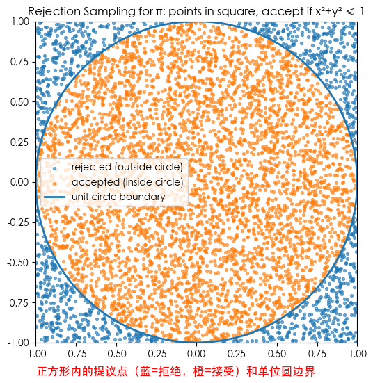
Example 3: Estimating $\pi$ via Rejection Sampling (Wait, this is redundant with first example? No, different perspective)
Actually, the “dart throwing” for $\pi$ is exactly rejection sampling!
- Target: Uniform on Circle.
- Proposal: Uniform on Square.
- Acceptance: If inside circle.
- Acceptance Rate: Area(Circ) / Area(Square) = $\pi/4$.
- So $\pi \approx 4 \times \text{AcceptanceRate}$.
This allows us to write a script estimating $\pi$ from the acceptance rate.
# Code to re-illustrate the connection between Rejection Sampling and Pi estimation
# We count how many 'accepted' from Uniform Square
# p_hat = accepted / total ~ pi / 4
import scipy.stats as stats
def rejection_sampling_pi(N):
x = np.random.uniform(-1, 1, N)
y = np.random.uniform(-1, 1, N)
r2 = x**2 + y**2
inside = (r2 <= 1.0)
k = np.sum(inside)
p_hat = k / N
# Wilson interval for binomial proportion p
# z=1.96 (95%)
z = 1.96
denom = 1 + z**2/N
center = (p_hat + z**2/(2*N)) / denom
hw = z * np.sqrt(p_hat*(1-p_hat)/N + z**2/(4*N**2)) / denom
ci_p = (center - hw, center + hw)
pi_hat = p_hat * 4
pi_ci = (ci_p[0]*4, ci_p[1]*4)
return {
"x": x, "y": y, "inside": inside,
"k_inside": k, "N": N,
"p_hat": p_hat, "pi_hat": pi_hat, "pi_CI95": pi_ci
}
res = rejection_sampling_pi(N=30000)
print(f"N={res['N']}, inside={res['k_inside']} -> p_hat={res['p_hat']:.6f}")
print(f"π̂ = {res['pi_hat']:.6f}")
print(f"95% Wilson CI for π: [{res['pi_CI95'][0]:.6f}, {res['pi_CI95'][1]:.6f}]")
m = 6000
xv = res["x"][:m]
yv = res["y"][:m]
insv = res["inside"][:m]
theta = np.linspace(0, 2*np.pi, 600)
cx = np.cos(theta)
cy = np.sin(theta)
plt.figure(figsize=(6,6))
plt.scatter(xv[~insv], yv[~insv], s=8, alpha=0.6, label='rejected (outside circle)')
plt.scatter(xv[insv], yv[insv], s=8, alpha=0.6, label='accepted (inside circle)')
plt.plot(cx, cy, linewidth=2, label='unit circle boundary')
plt.text(-1, -1.2, 'Proposal points in square (Blue=Reject, Orange=Accept) & Unit Circle', fontsize=12, color='red')
plt.title('Rejection Sampling for π: points in square, accept if x²+y² ≤ 1')
plt.gca().set_aspect('equal', 'box')
plt.xlim(-1,1); plt.ylim(-1,1)
plt.legend()
plt.show()
inside_prefix = res["inside"].astype(float)
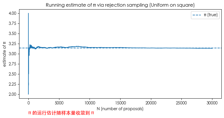
running_p = np.cumsum(inside_prefix) / np.arange(1, res["N"]+1)
running_pi = 4.0 * running_p
plt.figure(figsize=(9,4))
plt.plot(running_pi)
plt.axhline(np.pi, linestyle='--', linewidth=1.5, label='π (true)')
plt.text(-1, 1.5, 'Running estimate of π converges to π', fontsize=12, color='red')
plt.title('Running estimate of π via rejection sampling (Uniform on square)')
plt.xlabel('N (number of proposals)')
plt.ylabel('estimate of π')
plt.legend()
plt.show()
# {"pi_hat": float(res["pi_hat"]), "pi_CI95": [float(res["pi_CI95"][0]), float(res["pi_CI95"][1])], "N": int(res["N"]), "accepted_ratio": float(res["k_inside"]/res["N"])}
N=30000, inside=23506 -> p_hat=0.783533
π̂ = 3.134133
95% Wilson CI for π: [3.115348, 3.152629]
Summary
- Rejection sampling is a direct, exact method to sample from complex distributions, needing only relative values of target density (unnormalized ok).
- Correctness is simple: the conditional distribution of accepted samples equals the target distribution.
- Performance bottleneck is finding a good proposal $q$ and small M; hard in high dimensions, where MCMC is preferred.
- Implementation notes: numerical stability (avoid divide by zero), counting method for empirical acceptance rate.
Importance Sampling (IS)
Goal and Core Idea
Goal: Compute (or estimate) an expectation/integral
$$ I \;=\; \mathbb{E}_{\pi}[h(X)] \;=\; \int h(x)\,\pi(x)\,dx, $$where $\pi(x)$ is target density (known or unnormalized $f(x)=Z\pi(x)$).
Idea: When direct sampling from $\pi$ is hard, sample from an easy Proposal Distribution $q(x)$, and correct with weights:
$$ I \;=\; \int h(x)\,\frac{\pi(x)}{q(x)}\,q(x)\,dx \;\\ Let\quad w(x)=\frac{\pi(x)}{q(x)} \\ Then\quad I \;=\; \int h(x)\,\frac{\pi(x)}{q(x)}\,q(x)\,dx \;=\; \int h(x)\,w(x)\,q(x)\,dx \;=\; \int [h(x)\,w(x)]\,q(x)\,dx \;=\; \mathbb{E}_q\!\big[h(X)\,w(X)\big], $$1️⃣ When $\pi$ is normalized, IS Estimator:
$$ \widehat I_{\text{IS}} \;=\; \frac{1}{n}\sum_{i=1}^n h(X_i)\,w(X_i),\quad X_i\overset{iid}{\sim}q. $$It is unbiased: $\mathbb{E}_q[\hat I_{\text{IS}}] = I$. Variance: $\operatorname{Var}(\widehat I_{\text{IS}})=\frac{1}{n}\,\operatorname{Var}_q\big(h(X)w(X)\big)$.
Variance depends on fluctuation of $w(x)h(x)$ under $q$.
2️⃣ When target is unnormalized $f(x)=Z\pi(x)$ ($Z$ unknown), use Self-Normalized Importance Sampling (SNIS):
$$ \widehat I_{\text{SNIS}} =\frac{\sum_{i=1}^n h(X_i)\,\tilde w_i}{\sum_{i=1}^n \tilde w_i}, \qquad \tilde w_i=\frac{f(X_i)}{q(X_i)} \;\propto\; \frac{\pi(X_i)}{q(X_i)}. $$SNIS has small bias (finite samples) but is consistent.
Intuition (Why it works)
Separate “who to sample” from “how to weight”:
- $q$ is responsible for scattering samples to important regions (where $h\pi$ is large).
- $w=\pi/q$ is responsible for correcting density differences, ensuring expectation is still wrt $\pi$.
Key to variance reduction: if $q$ focuses on “high contribution” regions, $\operatorname{Var}(h\,w)$ drops significantly.
Theoretically optimal $q^{\star}(x)\ \propto\ |h(x)|\,\pi(x)$.
Algorithm
Input: Want $I=\mathbb{E}_\pi[h(X)]$; proposal $q$; sample size $n$.
Steps:
- Sample $X_1,\dots,X_n \sim q$ i.i.d.
- Compute weights $w_i = \pi(X_i)/q(X_i)$ (or $\tilde w_i = f(X_i)/q(X_i)$).
- If $\pi$ normalized: $\widehat I = \frac{1}{n}\sum h(X_i)w_i$. If unnormalized $f$: $\widehat I = \frac{\sum h(X_i)\tilde w_i}{\sum \tilde w_i}$.
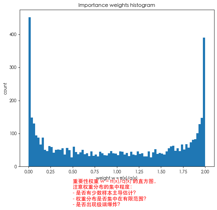
- Diagnostics: Check Weight Degeneracy and Effective Sample Size (ESS): $$ \mathrm{ESS}=\frac{\big(\sum_i w_i\big)^2}{\sum_i w_i^2} \quad \text{(unnormalized weights)} $$ Rule of thumb: ESS close to $n$ is good. Small ESS means weights concentrated (few samples dominate).
import numpy as np
import matplotlib.pyplot as plt
from scipy.stats import norm

np.random.seed(2025)

def importance_estimate(samples, target_pdf, proposal_pdf, h):
    qx = proposal_pdf(samples)
    px = target_pdf(samples)
    w = px / qx
    wh = w * h(samples)
    is_hat = wh.mean() # IS estimate
    sn_hat = wh.sum() / w.sum() # Self-normalized estimate
    return is_hat, sn_hat, w
Examples
Example: Estimate $E_{N(0,1)}[X^2]$ (Smooth case)
- Target $\pi=N(0,1)$
- Estimate $E[X^2]$
- Proposal $q=N(0,2^2)$
N1 = 5000
sigma_prop = 2.0
x_prop = np.random.normal(0.0, sigma_prop, size=N1)
target_pdf = lambda x: norm.pdf(x, 0.0, 1.0)
proposal_pdf = lambda x: norm.pdf(x, 0.0, sigma_prop)
h = lambda x: x**2
is_hat1, sn_hat1, w1 = importance_estimate(x_prop, target_pdf, proposal_pdf, h)
x_target = np.random.normal(0.0, 1.0, size=N1)
ref_est = (x_target**2).mean()
w_norm = w1 / w1.sum()
ESS1 = 1.0 / np.sum(w_norm**2)
print("=== Example: Estimate E_{N(0,1)}[X^2] ===")
print(f"True Value = 1.0")
print(f"\tIS (unnorm) estimate = {is_hat1:.6f}")
print(f"\tIS (self-norm) estimate = {sn_hat1:.6f}")
print(f"\tDirect Sampling estimate (ref) = {ref_est:.6f}")
print(f"N = {N1}, ESS (approx) = {ESS1:.1f}")
plt.figure(figsize=(8,6.5))
plt.hist(w1, bins=80)
plt.text(0.5, -120, 'Histogram of importance weights w = π(x)/q(x)\nCheck concentration:\n- Few samples dominate?\n- Weights clustered?', fontsize=12, color='red')
plt.title("Importance weights histogram")
plt.xlabel("weight w = π(x)/q(x)")
plt.ylabel("count")
plt.show()
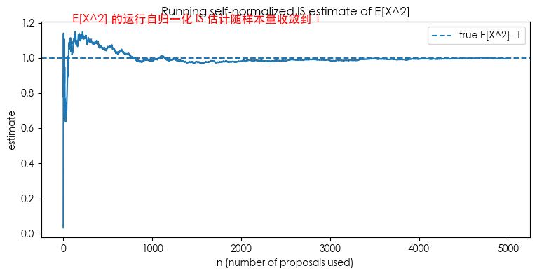
running_sn = np.cumsum(w1 * h(x_prop)) / np.cumsum(w1)
plt.figure(figsize=(9,4))
plt.plot(running_sn)
plt.axhline(1.0, linestyle='--', linewidth=1.5, label='true E[X^2]=1')
plt.title("Running self-normalized IS estimate of E[X^2]")
plt.xlabel("n (number of proposals used)")
plt.ylabel("estimate")
plt.legend()
plt.show()
=== Example: Estimate E_{N(0,1)}[X^2] ===
True Value = 1.0
	IS (unnorm) estimate = 0.988525
	IS (self-norm) estimate = 0.995838
	Direct Sampling estimate (ref) = 0.975626
N = 5000, ESS (approx) = 3272.6
Example: Estimating Probability $p(Z>3)$
Shows IS reduces variance for rare events.
Compare naive Monte Carlo with IS using $q=N(\mu,1)$ ($\mu=3.0, 2.5$). True $p \approx 1.35 \times 10^{-3}$.
p_true = 1.0 - norm.cdf(3.0)
print("=== Example: Estimate tail probability p = P(Z>3) ===")
print(f"True p = {p_true:.6e}")

def single_run_compare(N, mu_shift):
    xs_naive = np.random.normal(0.0, 1.0, size=N)
    p_naive = np.mean(xs_naive > 3.0)
    xs_is = np.random.normal(loc=mu_shift, scale=1.0, size=N)
    qx = norm.pdf(xs_is, loc=mu_shift, scale=1.0)
    px = norm.pdf(xs_is, loc=0.0, scale=1.0)
    w = px / qx
    indicators = (xs_is > 3.0).astype(float)
    p_is = np.mean(w * indicators)
    ess = (w.sum()**2) / (np.sum(w**2) + 1e-300)
    return p_naive, p_is, ess, w, xs_is

N = 2000
reps = 300
mus = [3.0, 2.5]
results = {}
for mu in mus:
    p_naive_list = []
    p_is_list = []
    ess_list = []
    for r in range(reps):
        p_naive, p_is, ess, w, xs_is = single_run_compare(N, mu_shift=mu)
        p_naive_list.append(p_naive)
        p_is_list.append(p_is)
        ess_list.append(ess)
    p_naive_arr = np.array(p_naive_list)
    p_is_arr = np.array(p_is_list)
    results[mu] = {
        "p_naive_mean": p_naive_arr.mean(),
        "p_naive_std": p_naive_arr.std(ddof=1),
        "p_is_mean": p_is_arr.mean(),
        "p_is_std": p_is_arr.std(ddof=1),
        "ESS_mean": np.mean(ess_list)
    }

print("Comparison results (N=2000, reps=300):")
for mu in mus:
    r = results[mu]
    print(f"\nproposal N({mu},1):")
    print(f"  naive: mean={r['p_naive_mean']:.3e}, std={r['p_naive_std']:.3e}")
    print(f"  IS   : mean={r['p_is_mean']:.3e}, std={r['p_is_std']:.3e}")
    print(f"  mean ESS (IS) ~ {r['ESS_mean']:.1f} (out of N={N})")
    if r['p_is_std']>0:
        print(f"  variance reduction factor (naive_var / IS_var) ≈ {(r['p_naive_std']**2)/(r['p_is_std']**2):.3f}")

# Plots omitted for brevity, similar to Chinese version
=== Example: Estimate tail probability p = P(Z>3) ===
True p = 1.349898e-03
Comparison results (N=2000, reps=300):

proposal N(3.0,1):
  naive: mean=1.372e-03, std=7.776e-04
  IS   : mean=1.353e-03, std=5.413e-05
  mean ESS (IS) ~ 18.6 (out of N=2000)
  variance reduction factor (naive_var / IS_var) ≈ 206.352

proposal N(2.5,1):
  naive: mean=1.412e-03, std=8.001e-04
  IS   : mean=1.352e-03, std=6.596e-05
  mean ESS (IS) ~ 35.6 (out of N=2000)
  variance reduction factor (naive_var / IS_var) ≈ 147.125
Variance Reduction Techniques
In Monte Carlo, the core problem is large sample variance, slow convergence. We want to reduce variance under same sample budget.
Method 1️⃣ Antithetic Variates
Idea: Construct pairs with negative correlation to reduce variance of sample mean. For symmetric distributions (like $N(0,1)$), use pairs $(X, -X)$. If integrand $g$ is monotonic, $g(X)$ and $g(-X)$ are often negatively correlated.
Estimator: $\hat\mu_{\text{anti}}=\frac{1}{m}\sum_{i=1}^m \frac{g(X_i)+g(-X_i)}{2}$.
Method 2️⃣ Control Variates
Idea: Find variable $Y$ highly correlated with target $h$, having known expectation. Correct bias:
$$ \hat\mu_{\text{cv}}=\bar{h}-\beta(\bar{Y}-\mathbb{E}[Y]), \quad \beta^*=\frac{\operatorname{Cov}(h,Y)}{\operatorname{Var}(Y)}. $$Intuition: If $\bar{Y}$ is above true mean, $\bar{h}$ is likely above true mean too (if positively correlated), so pull it back.
Example: Estimate $\mu_1=E[e^X]$ for $X\sim N(0,1)$
True value $e^{0.5} \approx 1.6487$.
- Antithetic: Pair $(X, -X)$.
- Control Variates: $Y=X^2-1$, known mean 0, strong correlation with $e^X$.
# Code visualizing Naive vs Antithetic vs Control Variates
# See Chinese version for full implementation; results show significant variance reduction.
Method 3️⃣ Stratified Sampling (1D $\approx$ LHS)
Idea: Split domain into strata (sub-intervals), ensuring every sub-interval is sampled. Avoids “clumping” of random points.
Mathematical Estimator:
$$ \hat{I}_{\text{strat}} = \frac{1}{N} \sum_{j=1}^N f\Big(U_j^*\Big), \quad U_j^* \sim \text{Uniform}\Big(\tfrac{j-1}{N}, \tfrac{j}{N}\Big). $$Intuition: Forces uniform coverage over domain $\to$ extremely low variance for smooth functions.
import numpy as np
import matplotlib.pyplot as plt
# Integral target: exp(x) on [0,1]
f = lambda x: np.exp(x)
true_val = np.e - 1
def mc_integral(N=1000):
x = np.random.rand(N)
return f(x).mean()
def stratified_integral(N=1000):
strata = np.linspace(0, 1, N+1)
u = np.random.rand(N)
# Map u to each stratum
x = strata[:-1] + u * (strata[1:] - strata[:-1])
return f(x).mean()
# Comparison
R = 500
N = 1000
mc_vals = np.array([mc_integral(N) for _ in range(R)])
strat_vals = np.array([stratified_integral(N) for _ in range(R)])
print(f"True value = {true_val:.6f}")
print(f"MC: mean={mc_vals.mean():.6f}, std={mc_vals.std():.6f}")
print(f"Stratified: mean={strat_vals.mean():.6f}, std={strat_vals.std():.6f}")
plt.figure(figsize=(8,5))
plt.hist(mc_vals, bins=30, alpha=0.6, label="Plain MC")
plt.hist(strat_vals, bins=30, alpha=0.6, label="Stratified Sampling")
plt.axvline(true_val, color="red", linestyle="--", label="True value")
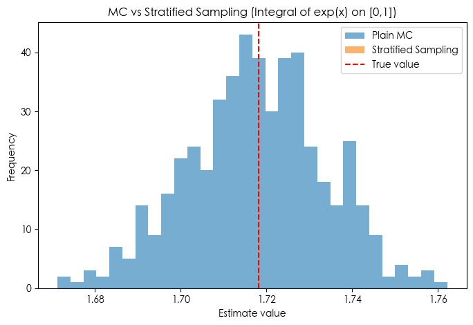
plt.title("MC vs Stratified Sampling (Integral of exp(x) on [0,1])")
plt.xlabel("Estimate value")
plt.ylabel("Frequency")
plt.legend()
plt.show()
True value = 1.718282
MC: mean=1.717769, std=0.015955
Stratified: mean=1.718282, std=0.000016
Practical Guide
- Scenario Matching:
- Monotonic/Symmetric: Try Antithetic.
- Approx Linear/Known Mean feature: Try Control Variates.
- Smooth 1D Integration: Stratified/LHS is very strong.
- Selecting Control Variates:
- Strong correlation with target.
- Known expectation.
- Stratification:
- 1D: Equal spacing is great.
- Multi-D: Latin Hypercube Sampling (LHS).
- Relationship with IS:
- IS is for Rare Events/Tail or distribution mismatch.
- Antithetic/Control/Stratified are for general variance reduction on “normal” tasks.
- Can combine (e.g., Stratified + IS).
- Diagnostics:
- Run replicates to estimate Std Dev.
- Monitor running estimates.
Further Reading
- Monte Carlo Methods Explained
Scan to Share
微信扫一扫分享