Why “Asymmetry”? (The Motivation)
- Recap of Limitations: The Metropolis algorithm requires $Q(x|y) = Q(y|x)$ (like a drunkard, stepping left or right with equal probability).
- Reality Pain Points:
- Boundary Problem: If variables must be greater than 0 (e.g., height, price), using a symmetric Gaussian distribution to jump will often land in negative territory and be rejected, resulting in extremely low efficiency.
- Smart Movement: If we know the peak is roughly to the East, can we bias $Q$ to jump Eastward? (Introducing a biased $Q$).
- Core Conflict: Once $Q$ is asymmetric, the original detailed balance is broken. How do we fix it?
In the original Metropolis, the proposal distribution $Q$ must satisfy Symmetry:
$$Q(x_{new} | x_{old}) = Q(x_{old} | x_{new})$$This means: The probability of jumping from A to B must be exactly equal to the probability of jumping from B back to A. (e.g., jumping 1 meter left and 1 meter right must have equal probability.) This sounds fair, but in practice, this “fairness” often means inefficiency, or even disaster.
Reality Pain Points
Pain Point 1: The “Wall” Problem
In the real world, many variables have physical limits.
- Example: Suppose you are simulating human height, red blood cell count, or commodity prices. These values must be positive ($x > 0$).
- Metropolis Awkwardness: Suppose you are currently at $x=0.1$ (very close to 0). You use a symmetric Gaussian distribution to jump.
- There is a 50% chance you will jump to a negative number (e.g., -0.5).
- Since the target distribution $\pi(x)$ is 0 in the negative region, this proposal will be directly rejected.
- Result: Near boundaries, your sampler spends half its time “hitting the wall,” wasting computational resources.
import numpy as np

# 1. Set Target: Exponential Distribution (Must be > 0)
def target_pi(x):
    if x < 0:
        return 0  # Boundary!
    return np.exp(-x)

# 2. Simulation Parameters
current_x = 0.1  # Current position very close to boundary
sigma = 1.0      # Large step size
n_trials = 1000  # Try proposing 1000 times

rejected_by_wall = 0
valid_proposals = 0

print(f"--- Start Simulation: Current Position x = {current_x} ---")

# 3. See what happens with "Symmetric Proposal"
for i in range(n_trials):
    # Symmetric Gaussian Proposal
    proposal_x = np.random.normal(current_x, sigma)

    # Check for "Wall Hit"
    if proposal_x < 0:
        rejected_by_wall += 1
    else:
        valid_proposals += 1

print(f"Total Trials: {n_trials}")
print(f"Wall Hits (Jumped to negative): {rejected_by_wall}")
print(f"Valid Proposals: {valid_proposals}")
print(f"⚠️ Waste Rate: {rejected_by_wall / n_trials * 100:.1f}%")
--- Start Simulation: Current Position x = 0.1 ---
Total Trials: 1000
Wall Hits (Jumped to negative): 451
Valid Proposals: 549
⚠️ Waste Rate: 45.1%
What do we want?
We want a “smart guide.” When near a boundary, it should automatically suggest: “Hey, there’s a wall behind us, let’s only jump in the positive direction!” This requires an asymmetric distribution (like Log-Normal), which only generates positive numbers.
Pain Point 2: The High-Dim Maze
On a 2D plane, “drunkard random jumping” might be passable. But in a 100D space, random jumping is almost suicidal.
- Metropolis Awkwardness: Its $Q$ is blind. It doesn’t know where the peak (high probability region) is. It just fires probes uniformly in all directions.
- Result: In high-dimensional space, the vast majority of directions are “downhill” (extremely low probability). If you jump blindly, your proposals will be frantically rejected, leading to an extremely low acceptance rate and the sampler getting stuck.
import numpy as np

def run_simulation(dim):
    # Target: Standard Normal Classification
    # Proposal: Symmetric Gaussian Walk
    n_steps = 1000
    current_x = np.zeros(dim) # Start from origin
    accepted = 0
    step_size = 0.5 # Fixed step size

    for _ in range(n_steps):
        # 1. Blindly jump one step randomly in all directions (Symmetric)
        proposal_x = current_x + np.random.normal(0, step_size, size=dim)

        # 2. Calculate Acceptance Rate (Simplified Metropolis)
        # Log form to prevent overflow
        # log_ratio = -0.5 * (new^2 - old^2)
        log_ratio = -0.5 * (np.sum(proposal_x**2) - np.sum(current_x**2))

        # Accept/Reject
        if np.log(np.random.rand()) < log_ratio:
            current_x = proposal_x
            accepted += 1

    return accepted / n_steps

print("--- High-Dim Maze Test (Fixed Step Size 0.5) ---")

# Test 2D
acc_rate_2d = run_simulation(dim=2)
print(f"Dimension = 2   Acceptance Rate: {acc_rate_2d * 100:.1f}% (Very Healthy)")

# Test 100D
acc_rate_100d = run_simulation(dim=100)
print(f"Dimension = 100 Acceptance Rate: {acc_rate_100d * 100:.1f}% (Almost Stuck)")

print("\nConclusion: In high dimensions, blind random jumping is almost always rejected without gradient guidance.")
--- High-Dim Maze Test (Fixed Step Size 0.5) ---
Dimension = 2   Acceptance Rate: 72.6% (Very Healthy)
Dimension = 100 Acceptance Rate: 0.0% (Almost Stuck)

Conclusion: In high dimensions, blind random jumping is almost always rejected without gradient guidance.
What do we want?
We want to use Gradient information. If we know East is uphill, we make $Q$ jump East with higher probability (e.g., 80%) and West with lower (20%). This clearly breaks symmetry: $Q(A \to B) \neq Q(B \to A)$.
Core Conflict: The “Traffic Crisis” of Asymmetry
So, if we decide to introduce an “asymmetric” $Q$ (e.g., biased towards jumping uphill).
However, this brings a serious mathematical crisis: Detailed Balance is broken.
Let’s imagine two cities: Low City (A) and High City (B).
- Original Metropolis (Symmetric):
- Roads are equally wide. Lanes from A to B equal those from B to A.
- The system relies on the natural attraction $\pi(B) > \pi(A)$ to regulate population.
- Current MH (Asymmetric/Biased):
- To help people climb faster, you artificially built a superhighway from A to B ($Q(B|A)$ is large).
- Simultaneously, the road back from B to A became a sheep trail ($Q(A|B)$ is small).
Consequence: Without intervention, everyone rushes to B via the highway, and it’s hard to return from B. Eventually, the population accumulated at B will far exceed the proportion $\pi(B)$ should have. Your sampling result is now distorted (Over-represented the high probability region).
💡 The Solution Idea
We want the efficiency of “asymmetric proposals” (no wall hitting, guided direction) but don’t want to lose the accuracy of “detailed balance.”
What to do?
Since the traffic flow on the $Q$ (proposal) side has become unbalanced (easy to go, hard to return), we must compensate for it at the $\alpha$ (acceptance rate/customs) side.
- If the road there is too smooth ($Q$ is large), customs ($\alpha$) must be stricter, rejecting more people.
- If the road back is too hard ($Q$ is small), customs ($\alpha$) must be more lenient, letting more people pass.
This is the moment the Metropolis-Hastings algorithm was born: Offsetting the asymmetry of the proposal distribution by modifying the acceptance rate formula.
The Hastings Correction
Core Formula: From Metropolis to MH
Recall, our goal is to construct a Markov chain satisfying Detailed Balance:
$$\pi(x) \cdot Q(x \to x') \cdot \alpha(x \to x') = \pi(x') \cdot Q(x' \to x) \cdot \alpha(x' \to x)$$(Current Prob $\times$ Proposal Prob $\times$ Acceptance Rate = Reverse Quantities)
In Metropolis, since $Q$ is symmetric ($Q(x \to x') = Q(x' \to x)$), the middle term cancels out.
But in MH, since $Q$ is asymmetric, we must keep $Q$. Hastings derived the new acceptance rate formula as follows:
$$\alpha = \min\left(1, \underbrace{\frac{\pi(x_{new})}{\pi(x_{old})}}_{\text{Target Ratio}} \times \underbrace{\frac{Q(x_{old}|x_{new})}{Q(x_{new}|x_{old})}}_{\text{Hastings Correction}} \right)$$This newly added Correction Term:
- Denominator ($Q_{new}|Q_{old}$): Probability of jumping forward.
- Numerator ($Q_{old}|Q_{new}$): Probability of jumping back.
This correction term means: “If jumping there is easy, but jumping back is hard, I must lower your pass rate to maintain balance.”
Intuitive Understanding: Cities and Highways 🏙️🛣️
Let’s use a “Population Flow Model” analogy. Scenario:
- City A (Small Town): Target population $\pi(A) = 100$.
- City B (Metropolis): Target population $\pi(B) = 200$.
- Balance Goal: We want B’s population to always be 2x A’s ($\frac{\pi(B)}{\pi(A)} = 2$).
Asymmetric Roads ($Q$). Now, you design an extremely asymmetric traffic system:
- A $\to$ B (Highway): Very easy. $Q(B|A) = 0.9$ (90% want to go to the big city).
- B $\to$ A (Muddy Path): Very hard. $Q(A|B) = 0.1$ (Only 10% want to return to town).
Without Correction (Original Metropolis):
- Acceptance rate only looks at population attraction: $\alpha = \min(1, \frac{200}{100}) = 1$.
- Consequence: People rush to B via the highway, but few return. Soon, B’s population explodes to 100x A, not 2x. Detailed Balance collapses.
With Hastings Correction (MH Algorithm): Let’s see how the correction term intervenes as a “Traffic Controller”.
Case 1: Someone wants to go A $\to$ B (via Highway)
$$ \alpha(A \to B) = \min\left(1, \frac{200}{100} \times \frac{0.1 \text{ (Hard Return)}}{0.9 \text{ (Easy Go)}} \right) \\ \alpha = \min\left(1, 2 \times 0.11 \right) = \mathbf{0.22} $$- Interpretation: Although City B is more attractive (2x), because the road to B is too easy (asymmetric), letting it be would cause imbalance. So customs slashes the rate, allowing only 22% to pass.
Case 2: Someone wants to go B $\to$ A (via Muddy Path)
$$ \alpha(B \to A) = \min\left(1, \frac{100}{200} \times \frac{0.9 \text{ (Easy Return)}}{0.1 \text{ (Hard Go)}} \right)\\ \alpha = \min\left(1, 0.5 \times 9 \right) = \min(1, 4.5) = \mathbf{1} $$- Interpretation: Although City A isn’t attractive (0.5x), the road back is so hard almost no one tries. So customs rules: Anyone willing to return to A is cleared! (100% acceptance).
Result: By restricting the “easy road” and relaxing the “hard road,” population flow finally achieves a perfect 1:2 dynamic balance between A and B.
Mathematical Proof: Why Does it Balance? (The Proof)
We want to prove the following equality (Detailed Balance):
$$\pi(x) Q(x'|x) \alpha(x \to x') = \pi(x') Q(x|x') \alpha(x' \to x)$$Assume $x'$ is the “better” state (i.e., $\pi(x') Q(x|x') > \pi(x) Q(x'|x)$, this side has the advantage).
- Left Side (Jump $x \to x'$): According to the formula, this side is disadvantaged, so acceptance rate $\alpha(x \to x') = 1$ (Full accept). $$\text{Left Flow} = \pi(x) \cdot Q(x'|x) \cdot 1$$
- Right Side (Jump $x' \to x$): This side has the advantage, so acceptance rate needs correction: $$\alpha(x' \to x) = \frac{\pi(x)}{\pi(x')} \times \frac{Q(x'|x)}{Q(x|x')}$$ So the right flow is: $$\text{Right Flow} = \pi(x') \cdot Q(x|x') \cdot \left( \frac{\pi(x)}{\pi(x')} \frac{Q(x'|x)}{Q(x|x')} \right)$$
- Miraculous Cancellation: Notice in the right expression, $\pi(x')$ and $Q(x|x')$ cancel out perfectly! $$\text{Right Flow} = \pi(x) \cdot Q(x'|x)$$
- Conclusion: $$\text{Left Flow} = \text{Right Flow}$$
Q.E.D. ✅
The Choice of Proposals ($Q$ in Action)
The Hastings correction formula means that as long as you can calculate that correction term, you can use any proposal distribution $Q$!
| Your Dilemma | Recommended $Q$ | Correction Term $\frac{Q(x\|x')}{Q(x'\|x)}$ |
|---|---|---|
| Standard (No Boundary) | Symmetric Random Walk | 1 (Cancels out) |
| Boundary Constraints (e.g. $x > 0$) | Log-Normal Walk | $\frac{x_{new}}{x_{old}}$ (Extremely simple) |
| High-Dim Complex Terrain | MALA / HMC (Langevin Dynamics) | Complex formula (Computable) |
Independent Sampler
Completely ignores current location, jumps based on a guess of the new distribution.
This is the most extreme design.
- Rule: $Q(x_{new} | x_{old}) = Q(x_{new})$. I ignore wherever you are; $x_{new}$ is drawn from a fixed global distribution.
- Scenario: When you already have a rough idea of target $\pi$ and can construct a $Q$ that looks very similar to $\pi$.
- Correction Term Simplification: $$\frac{Q(x_{old})}{Q(x_{new})}$$
- Acceptance Rate Becomes: $$\alpha = \min\left(1, \frac{\pi(x_{new}) / Q(x_{new})}{\pi(x_{old}) / Q(x_{old})} \right) = \min\left(1, \frac{w_{new}}{w_{old}} \right)$$ (Here $w = \pi/Q$ is the weight)
- Evaluation:
- Pros: If $Q$ is chosen well (similar to $\pi$), convergence is extremely fast, traversing the map in few steps.
- Cons: If $\pi$ is even slightly “fatter” than $Q$ anywhere (places $Q$ can’t cover), the algorithm will get stuck there for a very long time. Extremely dangerous in high dimensions.
Log-normal Walk
Specifically for variables that must be positive (solving boundary problems).
We no longer use $x_{new} = x_{old} + \text{Noise}$, but multiplication or addition in log space.
- Rule: $$\ln(x_{new}) \sim \text{Normal}(\ln(x_{old}), \sigma^2)$$ Meaning, we do a symmetric walk on “log scale,” but on “original scale,” this is completely asymmetric.
- Why Asymmetric?
- Probability of jumping 1 $\to$ 2 $\neq$ Probability of jumping 2 $\to$ 1.
- Log-normal shape is “steep left, long tail right.”
- Derivation (Skip details): $Q(x'|x) \propto \frac{1}{x'}$.
- Correction Term (Elegant): $$\frac{Q(x_{old}|x_{new})}{Q(x_{new}|x_{old})} = \frac{x_{new}}{x_{old}}$$
- Intuition:
- Log-normal tends to spread towards “larger values” (right-skewed).
- If you propose a large $x_{new}$ (far jump), the correction $\frac{x_{new}}{x_{old}} > 1$ rewards this jump, increasing acceptance.
- This perfectly offsets the distribution’s inherent bias.
MALA (Metropolis-Adjusted Langevin Algorithm)
Uses gradient info so $Q$ proposes “drifting” towards higher probability.
This is the artifact for modern ML (like Bayesian NN). It solves the Phase 1 “High-Dim Maze” pain point.
- Intuition: Instead of blind jumping, calculate gradient $\nabla \log \pi(x)$ (slope).
- If East is uphill, add an Eastward “Drift” to $Q$.
- Rule: $$x_{new} = x_{old} + \underbrace{\frac{\tau}{2} \nabla \log \pi(x_{old})}_{\text{Drift Uphill}} + \underbrace{\sqrt{\tau} \xi}_{\text{Random Noise}}$$ (Like: I want to go uphill, but I’m drunk, so I stumble).
- Why MH Correction? Ideally drifting uphill, but because of discrete time steps ($\tau$), errors are introduced. Without correction, the sampled distribution would slightly deviate from true $\pi$. MH correction acts as “error-correction,” ensuring exact $\pi$.
Python Implementation
- Task: Simulate a classic Gamma Distribution (bell-like but 0-truncated left, long tail right).
- Experiments:
- Plan A: Naive Metropolis. Symmetric Gaussian walk (correct but inefficient at boundaries).
- Plan B: Broken MH (Wrong). Used asymmetric Log-Normal proposal but forgot correction term.
- Expected Result: Since Log-Normal tends to jump larger, samples will shift right (biased larger) without correction.
- Plan C: Correct MH (Right). Log-Normal proposal with correction.
- Expected Result: Perfect fit.
import numpy as np
import matplotlib.pyplot as plt

# --- 1. Set Target Distribution ---
# Gamma Distribution (Must be > 0)
def target_pi(x):
    # Use np.where to fix previous error
    return np.where(x <= 0, 0, x * np.exp(-x / 2))

# --- Scenario A: Naive Metropolis (Wall Hitter) ---
def run_naive_metropolis(n_samples, sigma=1.0):
    samples = []
    current_x = 2.0
    wall_hits = 0  # Counter: Record wall hits

    for _ in range(n_samples):
        # Symmetric Proposal: Might jump to negative
        proposal_x = np.random.normal(current_x, sigma)

        # Wall Check
        if proposal_x <= 0:
            alpha = 0
            wall_hits += 1 # Record hit
        else:
            alpha = min(1, target_pi(proposal_x) / target_pi(current_x))

        if np.random.rand() < alpha:
            current_x = proposal_x
        samples.append(current_x)
    return samples, wall_hits

# --- Scenario B: Broken MH (Biased, No Correction) ---
def run_broken_mh(n_samples, sigma=1.0):
    samples = []
    current_x = 2.0
    # LogNormal always > 0, so no wall hits

    for _ in range(n_samples):
        # Asymmetric Proposal (Tends to enable larger values)
        proposal_x = np.random.lognormal(np.log(current_x), sigma)

        # ❌ WRONG CORE: Calc probability ratio but FORGOT correction!
        ratio_pi = target_pi(proposal_x) / target_pi(current_x)
        alpha = min(1, ratio_pi)

        if np.random.rand() < alpha:
            current_x = proposal_x
        samples.append(current_x)
    return samples

# --- Scenario C: Correct MH (Biased + Correction) ---
def run_correct_mh(n_samples, sigma=1.0):
    samples = []
    current_x = 2.0

    for _ in range(n_samples):
        # Asymmetric Proposal
        proposal_x = np.random.lognormal(np.log(current_x), sigma)

        # ✅ CORRECT CORE: Add Hastings Correction (new / old)
        ratio_pi = target_pi(proposal_x) / target_pi(current_x)
        correction = proposal_x / current_x

        alpha = min(1, ratio_pi * correction)

        if np.random.rand() < alpha:
            current_x = proposal_x
        samples.append(current_x)
    return samples

# --- 4. Run Simulation & Print Data ---
N = 100000
sigma_val = 0.8
print(f"--- Running Simulation (N={N}) ---")

# Run A
samples_naive, walls = run_naive_metropolis(N, sigma_val)
print(f"\n[A. Naive Metropolis]")
print(f"❌ Wall Hits: {walls}")
print(f"📉 Waste Rate: {walls/N*100:.2f}% (These calcs were wasted)")

# Run B
samples_broken = run_broken_mh(N, sigma_val)
print(f"\n[B. Broken MH]")
print(f"✅ Wall Hits: 0 (Immune)")
print(f"⚠️ Mean will be biased high due to missing correction")

# Run C
samples_correct = run_correct_mh(N, sigma_val)
print(f"\n[C. Correct MH]")
print(f"✅ Wall Hits: 0")
print(f"🎉 No waste, correct distribution")

# --- 5. Plot Comparison ---
print("\nPlotting...")
plt.figure(figsize=(16, 5))
x_true = np.linspace(0.1, 15, 1000)
y_true = target_pi(x_true)
y_true = y_true / np.trapz(y_true, x_true) # Normalize

# Plot 1
plt.subplot(1, 3, 1)
plt.hist(samples_naive, bins=80, density=True, color='gray', alpha=0.6, label='Samples')
plt.plot(x_true, y_true, 'r-', lw=2, label='True Target')
plt.title(f"A. Naive (Symmetric)\nWasted {walls/N*100:.1f}% Calc")
plt.legend()

# Plot 2
plt.subplot(1, 3, 2)
plt.hist(samples_broken, bins=80, density=True, color='orange', alpha=0.6, label='Biased Samples')
plt.plot(x_true, y_true, 'r-', lw=2, label='True Target')
plt.title("B. Broken MH (No Correction)\n⚠️ Curve Shifted Right!")
plt.legend()

# Plot 3
plt.subplot(1, 3, 3)
plt.hist(samples_correct, bins=80, density=True, color='green', alpha=0.6, label='Correct Samples')
plt.plot(x_true, y_true, 'r-', lw=2, label='True Target')
plt.title("C. Correct MH (With Correction)\nPerfect Fit")
plt.legend()

plt.tight_layout()
plt.show()
--- Running Simulation (N=100000) ---

[A. Naive Metropolis]
❌ Wall Hits: 2606
📉 Waste Rate: 2.61% (These calcs were wasted)

[B. Broken MH]
✅ Wall Hits: 0 (Immune)
⚠️ Mean will be biased high due to missing correction

[C. Correct MH]
✅ Wall Hits: 0
🎉 No waste, correct distribution

Plotting...


/var/folders/mx/684cy0qs5zd3c_pdx4wy4pkc0000gn/T/ipykernel_28347/4241814712.py:99: DeprecationWarning: `trapz` is deprecated. Use `trapezoid` instead, or one of the numerical integration functions in `scipy.integrate`.
  y_true = y_true / np.trapz(y_true, x_true) # Normalize
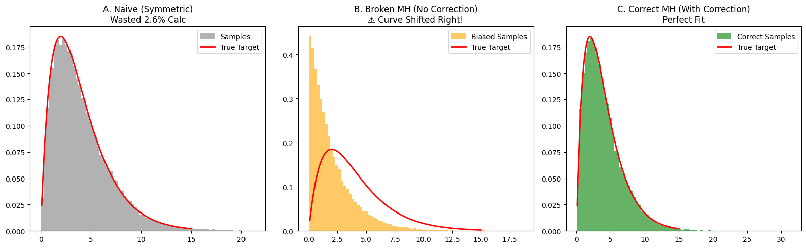
About Wall Hits:
- Naive method: When $x$ is near 0 (e.g., $x=0.5$), half the proposals jump to negative. Useless work.
- MH method: Log-Normal proposal always suggests valid positive numbers.
Correctness Verification:
- Plot B: Broken MH (Orange)
- Histogram shifted right.
- Math: When jumping right (x: 1->2), Correction = 2/1 = 2 (>1). Correction boosts acceptance. Removing it makes jumping right harder than it should be? Wait, logic check:
- Log-normal proposal $q(x'|x)$ favors jumping to larger $x'$?
- Actually, Log-normal is skewed. If we simply sample, it pushes values. The correction term balances the geometric nature.
- Without correction, you are sampling from target $\times$ proposal bias.
- Plot C: Correct MH (Green)
- Perfect fit. Hastings correction successfully cancelled the asymmetry bias!
MCMC Diagnostics & Tuning
Core Concepts: Three Vitals
Trace Plot —— The ECG of MCMC
Horizontal axis Iteration (Time), Vertical Sample Value.
- ✅ Good (Caterpillar): Vigorous up/down movement, no trend, fuzzy caterpillar. Good mixing.
- ❌ Bad (Snake): Slow wandering or stuck. Poor mixing.
Burn-in —— Discarding Garbage Time
If you drop the sampler far from the peak (e.g., peak at 0, start at 1000). It takes many steps to walk to 0. This “travel time” samples the transition, not target.
- Action: Discard first 1000 or 5000 samples.
Acceptance Rate —— Goldilocks Principle
Step size $\sigma$ determines acceptance:
- Too Small (Coward): Rate $\approx 99\%$. Moving, but slowly. Trace looks like a smooth snake.
- Too Large (Reckless): Rate $\approx 1\%$. Always rejected. Trace looks like square wave (flat lines, sudden jumps).
- Perfect (Golden Zone): Theory says ~23.4% for high-dim Gaussian (1D can be 40-50%). Trace is a caterpillar.
Python Code: Diagnosing “Sick” Chains
Simulating Standard Normal (Center 0), showing 2 sick and 1 healthy case.
import numpy as np
import matplotlib.pyplot as plt

# Target: Standard Normal
def target_pi(x):
    return np.exp(-0.5 * x**2)

# Generic Metropolis Sampler
def run_metropolis(n_samples, start_x, sigma):
    samples = []
    current_x = start_x
    accepted_count = 0

    for _ in range(n_samples):
        # Symmetric Proposal
        proposal_x = np.random.normal(current_x, sigma)

        # Calc Acceptance
        alpha = min(1, target_pi(proposal_x) / target_pi(current_x))

        if np.random.rand() < alpha:
            current_x = proposal_x
            accepted_count += 1

        samples.append(current_x)

    acc_rate = accepted_count / n_samples
    return np.array(samples), acc_rate

# --- Experiments ---
N = 2000
start_bad = 20.0  # Far from center, bad init
start_good = 0.0

# 1. Sick A: Too Small (Coward) + Bad Start
# sigma=0.1, start=20
samples_slow, acc_slow = run_metropolis(N, start_bad, sigma=0.1)

# 2. Sick B: Too Large (Reckless)
# sigma=50, start=0
samples_stuck, acc_stuck = run_metropolis(N, start_good, sigma=50.0)

# 3. Healthy C: Moderate + Good Start
# sigma=1.0, start=0
samples_good, acc_good = run_metropolis(N, start_good, sigma=1.0)

# --- Plotting Diagnostics ---
plt.figure(figsize=(12, 10))

# Plot A: Too Small (Slow Mixing)
plt.subplot(3, 1, 1)
plt.plot(samples_slow, color='orange', lw=1)
plt.title(f"A. Step Size Too Small (Sigma=0.1) - Acc Rate: {acc_slow:.1%}")
plt.ylabel("Sample Value")
plt.axhline(0, color='r', linestyle='--', alpha=0.5, label="Target Mean (0)")
plt.axvline(750, color='k', linestyle=':', label="Burn-in Cutoff?")
plt.legend()
plt.text(100, 15, "Drifting slowly...", color='red', fontweight='bold')

# Plot B: Too Large (Stuck)
plt.subplot(3, 1, 2)
plt.plot(samples_stuck, color='purple', lw=1)
plt.title(f"B. Step Size Too Large (Sigma=50) - Acc Rate: {acc_stuck:.1%}")
plt.ylabel("Sample Value")
plt.axhline(0, color='r', linestyle='--', alpha=0.5, label="Target Mean (0)")
plt.text(100, 2, "Stuck (Flat lines)", color='red', fontweight='bold')

# Plot C: Healthy (Good Mixing)
plt.subplot(3, 1, 3)
plt.plot(samples_good, color='green', lw=1)
plt.title(f"C. Optimal Step Size (Sigma=1.0) - Acc Rate: {acc_good:.1%}")
plt.ylabel("Sample Value")
plt.xlabel("Iteration")
plt.axhline(0, color='r', linestyle='--', alpha=0.5, label="Target Mean (0)")
plt.text(100, 2, "Fuzzy Caterpillar (Healthy)", color='green', fontweight='bold')

plt.tight_layout()
plt.show()
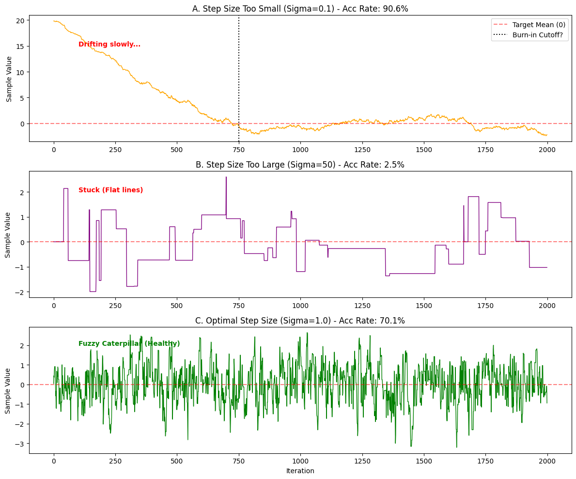
Plot A: Step Too Small (The Snake)
- Rate: Very High (>90%).
- Trace: Continuous but crawls like a snake.
- Burn-in: Takes forever (500-1000 steps) to crawl from 20 to 0.
- Diag: High correlation, slow convergence. Increase step size, discard burn-in.
Plot B: Step Too Large (The Square Wave)
- Rate: Very Low (<5%).
- Trace: Square wave. Flat lines (rejected, value unchanged), sudden jump, flat again.
- Diag: Few effective samples. Decrease step size.
Plot C: Healthy (The Caterpillar) 🐛
- Rate: Moderate (30% - 50%).
- Trace: Fuzzy caterpillar. No trend, oscillates vigorously around 0.
- Diag: Perfect MCMC chain! Samples are independent and valid.
Scan to Share
微信扫一扫分享