What Problem Are We Trying to Solve? (The Core Problem)
1. The Core Dilemma: Intractable $Z$
In Bayesian statistics, physics simulations, and high-dimensional computing, we often need to sample from a complex probability distribution $\pi(x)$. However, we typically only know the “shape” of this distribution, but not its “scale”.
- Known: Unnormalized density function $f(x)$ (relative weights).
- Unknown: Normalization constant $Z$ (total sum or integral). $$\pi(x) = \frac{f(x)}{Z}, \quad \text{where } Z = \int f(x) dx$$
- Pain Point: In high-dimensional spaces, calculating $Z$ (summing over the entire space) is computationally intractable.
- Consequence: Because we don’t know $Z$, we cannot calculate the absolute probability $\pi(x)$, and traditional direct sampling methods (like inverse transform sampling) fail completely.
About $\pi$
| Scenario | Form of $\pi$ | Mathematical Name | Physical Meaning |
|---|---|---|---|
| Basic Markov Chains | Vector | Stationary Distribution Vector | Long-term probability of being in each state |
| Metropolis (MCMC) | Function | Target Probability Density | The “shape” we want to sample from |
2. Metropolis Strategy: Relative Ratios
The core insight of the Metropolis algorithm is: Since we can’t calculate $Z$, let’s cancel it out.
Instead of calculating absolute probabilities, if we compare the relative probability ratio between two states, the constant $Z$ automatically cancels out in the numerator and denominator:
$$\frac{\pi(x_{\text{new}})}{\pi(x_{\text{old}})} = \frac{f(x_{\text{new}}) / Z}{f(x_{\text{old}}) / Z} = \frac{f(x_{\text{new}})}{f(x_{\text{old}})}$$This allows us to judge the superiority of two states using only relative heights (ratio of $f(x)$), thereby bypassing the difficulty of calculating $Z$.
3. Connection: Why Use Markov Chains?
Since we can only make “local comparisons” (comparing current position with next position), we cannot generate independent samples in one go. We need a mechanism to wander through the space, which introduces Markov chains.
Simulating Static with Dynamic: Our goal is to obtain samples from a static distribution $\pi$. The Metropolis method constructs a dynamic process (Markov chain) to do this.
Reverse Engineering Mindset:
- Traditional Markov Chain Problem: Given transition matrix $P$, find stationary distribution $\pi$.
- Metropolis (MCMC) Problem: Given target distribution $\pi$, design a transition matrix $P$ such that the chain eventually converges to $\pi$.
Algorithm Essence: The Metropolis algorithm constructs a special “accept/reject” rule via Detailed Balance Principle, generating an HIA chain (Homogeneous, Irreducible, Aperiodic) on the fly.
Final Conclusion: According to the Ergodic Theorem, the trajectory generated by this Markov chain is statistically equivalent to samples drawn from the target distribution $Z$ in the long run.
One-sentence Summary: The Metropolis algorithm is designed to solve the problem of “sampling when the normalization constant $Z$ is unknown” by “constructing a Markov chain with the target distribution as its stationary state”.
Metropolis (Random Walk)
To ensure convergence to $\pi$, we just need to construct a chain that satisfies the Detailed Balance Equation:
$$\pi_i P_{ij} = \pi_j P_{ji}$$The Metropolis algorithm splits the transition process into two steps:
- Proposal $Q_{ij}$: In mathematical notation, it is often written as $Q(x_{new} | x_{old})$ or $q(x' | x)$. It means: “Given I am at $x_{old}$, what is the probability I propose to jump to $x_{new}$?”
- Note it’s called “Proposal”. It only suggests: “Hey, should we try going there?” Whether we actually go is determined by $\alpha$ (acceptance rate) later.
- In the original Metropolis algorithm, $Q$ must be Symmetric: $$Q(x_{new} | x_{old}) = Q(x_{old} | x_{new})$$
- This allows us to cancel $Q$ out when calculating acceptance rate later.
- In practice, $Q$ is usually a simple line of random number generation code. Two common forms:
- A. Uniform Random Walk
- Code:
x_new = x_old + random.uniform(-1, 1) - Logic: Draw a box of width 2 centered at current position, any point inside has equal probability.
- Feature: Simple and crude.
- Code:
- B. Gaussian Random Walk
- Code:
x_new = x_old + random.normal(0, sigma) - Logic: Generate a normal distribution centered at current position. Closer points are more likely proposed.
- Feature: Mimics natural movement (mostly small steps, occasionally large steps).
- Code:
- A. Uniform Random Walk
- Acceptance $\alpha_{ij}$: Decides “Do I really jump there, or stay put?”.
- Although acceptance rate is a fixed value determined by state pair $(i, j)$, in engineering, since state count $N$ is astronomical, we can never pre-calculate and store this $N \times N$ table. We can only “calculate as we go”.
- ⚠️ The entire reason Metropolis algorithm exists is because the state space is too large (or continuous infinite), making it impossible to pre-determine this “2D array” of acceptance rates.
So, the actual transition probability is: $P_{ij} = Q_{ij} \times \alpha_{ij}$. Substitute into detailed balance equation:
$$\pi_i (Q_{ij} \alpha_{ij}) = \pi_j (Q_{ji} \alpha_{ji})$$Assuming we use a symmetric proposal rule (i.e., $Q_{ij} = Q_{ji}$, e.g., jumping left and right has same probability). The equation simplifies to:
$$\pi_i \alpha_{ij} = \pi_j \alpha_{ji}$$Or as a ratio:
$$\frac{\alpha_{ij}}{\alpha_{ji}} = \frac{\pi_j}{\pi_i}$$Suppose you are at state $i$, system suggests jumping to state $j$. If state $j$ has higher probability than state $i$ (i.e., $\pi_j > \pi_i$, moving “uphill”), to satisfy the ratio above, acceptance probability $\alpha_{ij}$ should be set to 1 (100%) for maximum efficiency. Since $\pi_j > \pi_i$, new state $j$ is “better” or “more important”, we are happy to move uphill, so we accept without hesitation.
This gives the famous Metropolis Acceptance Probability:
$$\alpha_{ij} = \min \left( 1, \frac{\pi_j}{\pi_i} \right)$$It covers two cases:
- Moving uphill ($\pi_j > \pi_i$): Ratio $>1$, $\min$ gives 1. Always accept.
- Moving downhill ($\pi_j < \pi_i$): Ratio $<1$, $\min$ gives $\frac{\pi_j}{\pi_i}$.
- This is the soul of the algorithm!
- Even if the new state is worse, we still accept it with some probability (though not 100%).
- Why? To prevent getting stuck in “Local Optima”. Occasionally accepting bad results allows jumping out of small pits to search for higher peaks further away.
import numpy as np
import matplotlib.pyplot as plt
# 1. Define Target Distribution pi(x)
# Here we use standard normal: proportional to exp(-0.5 * x^2)
def target_pi(x):
return np.exp(-0.5 * x**2)
# 2. Metropolis Algorithm Settings
num_samples = 100000
current_state = 0 # Arbitrary start
samples = []
# 3. Start Sampling Loop
for _ in range(num_samples):
# A. Proposal: Random jump near current position
# Q(j|i) is symmetric (e.g. using uniform or gaussian as jump step)
proposal_state = current_state + np.random.uniform(-1, 1)
# B. Calculate Acceptance Probability
# alpha = min(1, pi_new / pi_old)
ratio = target_pi(proposal_state) / target_pi(current_state)
acceptance_prob = min(1, ratio)
# C. Decide to Move (Accept/Reject Step)
# Generate 0-1 random number, accept if less than acceptance prob
if np.random.rand() < acceptance_prob:
current_state = proposal_state # Move to new position
# Record current position whether accepted or rejected (Note: if rejected, record old position!)
samples.append(current_state)
# --- Plot Verification ---
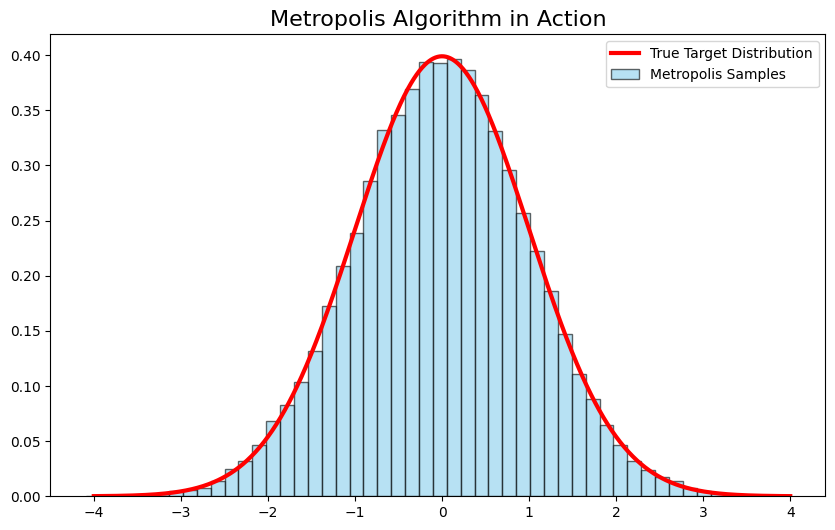
plt.figure(figsize=(10, 6))
# Plot True Curve (Theoretical)
x = np.linspace(-4, 4, 1000)
plt.plot(x, target_pi(x) / np.sqrt(2 * np.pi), 'r-', lw=3, label='True Target Distribution')
# Plot Histogram from Metropolis Sampling
plt.hist(samples, bins=50, density=True, alpha=0.6, color='skyblue', edgecolor='black', label='Metropolis Samples')
plt.title("Metropolis Algorithm in Action", fontsize=16)
plt.legend()
plt.show()
One-Dimensional case
Input:
- Target (unnormalized) log density $\log \tilde\pi(x)$
- Initial point $x_0$
- Symmetric proposal distribution $q(y\mid x)=\mathcal N(x,\sigma^2)$ (multivariate normal for high dim)
- Total steps $T$, discard first $B$ steps as burn-in
Each Step $t=0,1,2,\dots,T-1$:
- Propose from symmetric proposal: $y \sim \mathcal N(x_t,\sigma^2)$.
- Calculate Acceptance Rate:
Note we only use the ratio, no normalization constant needed! For numerical stability, use $\log\tilde\pi$: $\log\alpha = \min\{0,\ \log\tilde\pi(y)-\log\tilde\pi(x_t)\}$.
- Accept with probability $\alpha$: $x_{t+1}=y$; Else reject: $x_{t+1}=x_t$.
Output:
- Sample sequence after discarding first $B$ steps as approximate samples from $\pi$;
- Report Acceptance Rate (accepted count / total steps).
Correctness Explanation
Core is Detailed Balance (Reversibility): With symmetric proposal $q(y\mid x)=q(x\mid y)$, Metropolis acceptance rate ensures
$$ \pi(x)\,q(y\mid x)\,\alpha(x,y)=\pi(y)\,q(x\mid y)\,\alpha(y,x), $$Thus $\pi$ is the Stationary Distribution (invariant distribution). As long as the chain is also Irreducible + Aperiodic, it will converge to $\pi$ from any start point (in TV distance).
Intuition: Balance the probability flow “from $x$ to $y$” exactly with “from $y$ to $x$” at each step, so there is no net flow in long term, stabilizing at $\pi$.
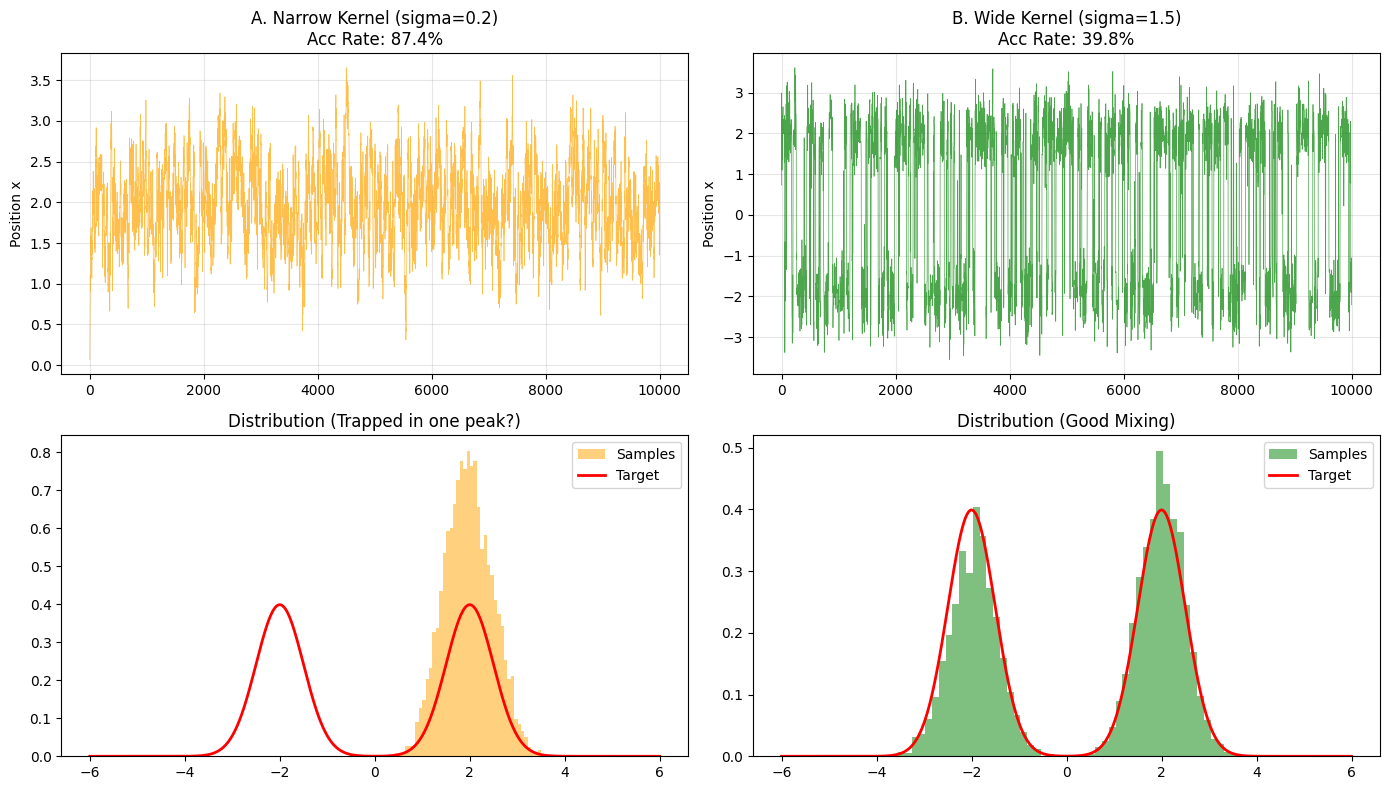
$\sigma$ (Step Size)
- $\sigma$ Too Small: Almost always accept, but moves very slowly, samples strongly correlated, Low ESS;
- $\sigma$ Too Large: Often propose to low density areas, high rejection, inefficient;
- $\sigma$ Appropriate: Good tradeoff between acceptance and move size, fast ACF decay, High ESS.
Empirically: For Random Walk Metropolis, optimal acceptance rate is around ~0.4 for 1D; for higher dimensions, 0.2–0.3 is common (rule of thumb, not law).
Example
import numpy as np
import pandas as pd
import matplotlib.pyplot as plt

rng = np.random.default_rng(123)

def acf_1d(x, max_lag=200):
    x = np.asarray(x)
    x = x - np.mean(x) # zero-mean
    n = len(x)
    var = np.var(x) # biased variance
    out = np.empty(max_lag+1, dtype=float)
    out[0] = 1.0
    for k in range(1, max_lag+1):
        out[k] = np.dot(x[:-k], x[k:]) / ((n-k) * var)
    return out

def ess_from_acf(acf_vals, n):
    s = 0.0
    for k in range(1, len(acf_vals)):
        if acf_vals[k] <= 0:
            break
        s += 2 * acf_vals[k]
    tau_int = 1.0 + s
    return n / tau_int

def normalize_pdf(xs, logpdf):
    lps = np.array([logpdf(x) for x in xs])
    lps -= np.max(lps)
    pdf_unnorm = np.exp(lps)
    Z = np.trapezoid(pdf_unnorm, xs)
    return pdf_unnorm / Z

def metropolis(logpdf, x0, proposal_std, n_steps, burn_in=0, rng=None):
    """Metropolis algorithm for 1D distributions.

    Args:
        logpdf: function that computes the log of the target PDF at a given x
        x0: initial position (float)
        proposal_std: standard deviation of the Gaussian proposal distribution (float)
        n_steps: total number of MCMC steps (int)
        burn_in: number of initial samples to discard (int, default=0)
        rng: optional numpy random generator (default=None, uses np.random.default_rng())
    """
    if rng is None:
        local_rng = np.random.default_rng()
    else:
        local_rng = rng
    x = float(x0)
    samples = []
    accepted = 0
    accepts = []
    for t in range(n_steps): # t = 0, 1, ..., n_steps-1
        y = x + local_rng.normal(0.0, proposal_std) # propose new position
        logacc = logpdf(y) - logpdf(x) # log acceptance ratio
        if np.log(local_rng.uniform()) < logacc: # accept/reject
            x = y
            accepted += 1
            accepts.append(1)
        else:
            accepts.append(0)
        if t >= burn_in: # record sample after burn-in
            samples.append(x)
    acc_rate = accepted / n_steps # acceptance rate
    return np.array(samples), acc_rate, np.array(accepts)
Unimodal Example
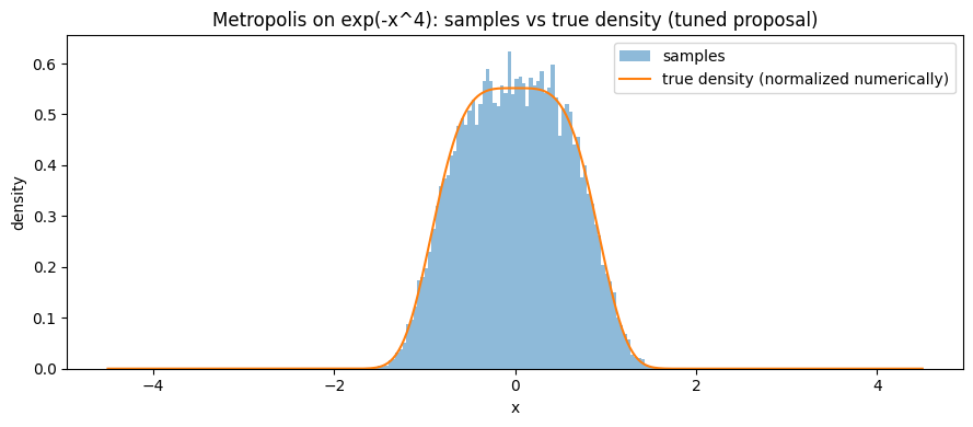
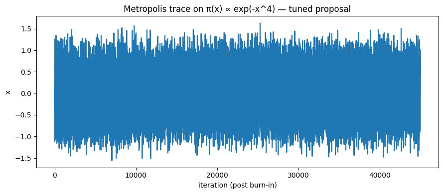
Unimodal hard-to-normalize distribution: $\pi(x)\propto e^{-x^4}$
Observe acceptance rate, ACF, ESS, histogram vs true density (numerically normalized) under different $\sigma$.
import os
# Example : exp(-x^4)
def logpdf_expfour(x):
return - (x**4)
save_folder = "./mcmc_meetropolis_results"
os.makedirs(save_folder, exist_ok=True)
n_steps = 50000
burn_in = 5000
x0 = 0.0
configs = [("small", 0.15), ("tuned", 0.8), ("large", 3.0)]
results_A = []
for name, s in configs:
samples, acc_rate, accepts = metropolis(logpdf_expfour, x0, s, n_steps, burn_in, rng)
acf_vals = acf_1d(samples, max_lag=200)
ess = ess_from_acf(acf_vals, len(samples))
results_A.append({"config": name, "proposal_std": s, "accept_rate": acc_rate, "ESS": ess, "n_kept": len(samples)})
pd.DataFrame({"x": samples}).to_csv(f"{save_folder}/metropolis_expfour_{name}.csv", index=False)
samples_tuned = pd.read_csv(f"{save_folder}/metropolis_expfour_tuned.csv")["x"].values
plt.figure(figsize=(9,4))
plt.plot(samples_tuned)
plt.xlabel("iteration (post burn-in)")
plt.ylabel("x")
plt.title("Metropolis trace on π(x) ∝ exp(-x^4) — tuned proposal")
plt.tight_layout()
plt.savefig(f"{save_folder}/expfour_trace_tuned.png", dpi=150)
plt.show()
xs = np.linspace(-4.5, 4.5, 600)
true_pdf = normalize_pdf(xs, logpdf_expfour)
plt.figure(figsize=(9,4))
plt.hist(samples_tuned, bins=80, density=True, alpha=0.5, label="samples")
plt.plot(xs, true_pdf, label="true density (normalized numerically)")
plt.xlabel("x")
plt.ylabel("density")
plt.title("Metropolis on exp(-x^4): samples vs true density (tuned proposal)")
plt.legend()
plt.tight_layout()
plt.savefig(f"{save_folder}/expfour_hist_tuned.png", dpi=150)
plt.show()
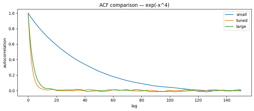
plt.figure(figsize=(9,4))
for name, _ in configs:
x = pd.read_csv(f"{save_folder}/metropolis_expfour_{name}.csv")["x"].values
acf_vals = acf_1d(x, max_lag=150)
plt.plot(acf_vals, label=f"{name}")
plt.xlabel("lag")
plt.ylabel("autocorrelation")
plt.title("ACF comparison — exp(-x^4)")
plt.legend()
plt.tight_layout()
plt.savefig(f"{save_folder}/expfour_acf_compare.png", dpi=150)
plt.show()
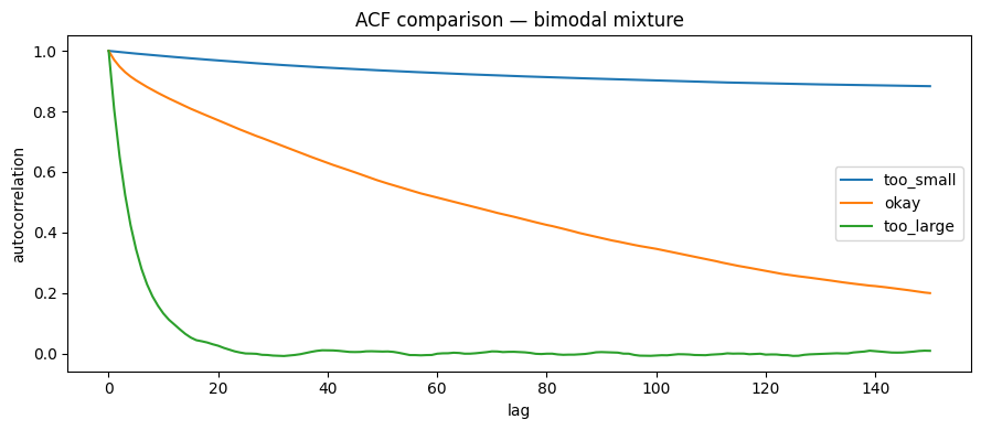
Bimodal Example
Bimodal Mixture: 0.5 $\mathcal N(-3,1)$ + 0.5 $\mathcal N(3,1)$
Observe “mode trapping” of random walk in multi-modal terrain, and counter-examples of $\sigma$ too small/large.
# Example: bimodal mixture
import os
save_folder = "./mcmc_meetropolis_results"
os.makedirs(save_folder, exist_ok=True)
def logpdf_bimodal(x):
    mu1, mu2, s = -3.0, 3.0, 1.0
    l1 = -0.5*((x-mu1)/s)**2 - 0.5*np.log(2*np.pi*s*s) + np.log(0.5)
    l2 = -0.5*((x-mu2)/s)**2 - 0.5*np.log(2*np.pi*s*s) + np.log(0.5)
    m = np.maximum(l1, l2)
    return m + np.log(np.exp(l1-m) + np.exp(l2-m))

configs_B = [("too_small", 0.2), ("okay", 1.2), ("too_large", 4.0)]
results_B = []
for name, s in configs_B:
    samples, acc_rate, accepts = metropolis(logpdf_bimodal, x0=-5.0, proposal_std=s, n_steps=n_steps, burn_in=burn_in, rng=rng)
    acf_vals = acf_1d(samples, max_lag=200)
    ess = ess_from_acf(acf_vals, len(samples))
    frac_right = float(np.mean(samples > 0))
    results_B.append({"config": name, "proposal_std": s, "accept_rate": acc_rate, "ESS": ess, "frac_right_mode": frac_right, "n_kept": len(samples)})
    pd.DataFrame({"x": samples}).to_csv(f"{save_folder}/metropolis_bimodal_{name}.csv", index=False)

xs2 = np.linspace(-8, 8, 700)
pdf2 = normalize_pdf(xs2, logpdf_bimodal)
samples_ok = pd.read_csv(f"{save_folder}/metropolis_bimodal_okay.csv")["x"].values
plt.figure(figsize=(9,4))
plt.hist(samples_ok, bins=120, density=True, alpha=0.5, label="samples (okay)")
plt.plot(xs2, pdf2, label="true density (normalized numerically)")
plt.xlabel("x")
plt.ylabel("density")
plt.title("Metropolis on bimodal mixture — histogram vs true density")
plt.legend()
plt.tight_layout()
plt.savefig(f"{save_folder}/bimodal_hist_okay.png", dpi=150)
plt.show()

plt.figure(figsize=(9,4))
for name, _ in configs_B:
    x = pd.read_csv(f"{save_folder}/metropolis_bimodal_{name}.csv")["x"].values
    acf_vals = acf_1d(x, max_lag=150)
    plt.plot(acf_vals, label=name)
plt.xlabel("lag")
plt.ylabel("autocorrelation")
plt.title("ACF comparison — bimodal mixture")
plt.legend()
plt.tight_layout()
plt.savefig(f"{save_folder}/bimodal_acf_compare.png", dpi=150)
plt.show()

2D/High-Dim Version: Correlated Gaussian
Intuition:
- Challenges of Random Walk Metropolis in High Dimensions;
- Impact of proposal covariance scaling on acceptance rate and ESS.
Target Distribution: 2D Correlated Gaussian
Target distribution:
$$ \pi(x) = \mathcal N\Big(0, \Sigma\Big),\quad \Sigma = \begin{bmatrix}1 & 0.8\\0.8 & 1\end{bmatrix}. $$This is an “elliptical” 2D Gaussian, main direction along $y=x$.
Metropolis Settings
Proposal Distribution: Symmetric Gaussian
$$ q(y\mid x) = \mathcal N(x,\, \sigma^2 I). $$We compare three $\sigma$:
- Too Small (0.05)
- Appropriate (0.5)
- Too Large (2.0)
Diagnostics
- Acceptance Rate (accepted / total steps)
- ESS (Effective Sample Size): Estimated approximately for each dimension using autocorrelation
- Trace/Scatter: Observe if exploring along ellipse major axis
- ACF: Compare decay speed of different $\sigma$
import numpy as np
import matplotlib.pyplot as plt

# ---------- Target Distribution (2D Correlated Gaussian) ----------
Sigma = np.array([[1.0, 0.8],
                  [0.8, 1.0]])
Sigma_inv = np.linalg.inv(Sigma)
Sigma_det = np.linalg.det(Sigma)
d = 2

def log_target(x):
    # log density of N(0, Sigma)
    return -0.5 * x @ Sigma_inv @ x

# ---------- Metropolis Implementation ----------
def metropolis_2d(log_target, x0, sigma, n_samples=20000, burn_in=2000):
    x = np.zeros((n_samples, d))
    x[0] = x0
    accepted = 0
    for t in range(1, n_samples):
        proposal = x[t-1] + sigma * np.random.randn(d)
        log_alpha = log_target(proposal) - log_target(x[t-1])
        if np.log(np.random.rand()) < log_alpha:
            x[t] = proposal
            accepted += 1
        else:
            x[t] = x[t-1]
    return x[burn_in:], accepted/(n_samples-1)

# ---------- Autocorrelation & ESS ----------
def autocorr(x, lag):
    n = len(x)
    x_mean = np.mean(x)
    num = np.sum((x[:n-lag]-x_mean)*(x[lag:]-x_mean))
    den = np.sum((x-x_mean)**2)
    return num/den

def ess(x):
    # Simple approx ESS = N / (1 + 2*sum_rho)
    n = len(x)
    acfs = []
    for lag in range(1, 200):  # Truncate at 200 lags
        r = autocorr(x, lag)
        if r <= 0:
            break
        acfs.append(r)
    tau = 1 + 2*np.sum(acfs)
    return n/tau

# ---------- Run different sigma ----------
sigmas = [0.05, 0.5, 2.0]
results = {}

for sigma in sigmas:
    samples, acc_rate = metropolis_2d(log_target, np.zeros(d), sigma)
    ess_x = ess(samples[:,0])
    ess_y = ess(samples[:,1])
    results[sigma] = {
        "samples": samples,
        "acc_rate": acc_rate,
        "ESS_x": ess_x,
        "ESS_y": ess_y
    }

# ---------- Plot: Scatter & Trace ----------
fig, axes = plt.subplots(1, 3, figsize=(15,5))
for ax, sigma in zip(axes, sigmas):
    s = results[sigma]["samples"]
    ax.scatter(s[:,0], s[:,1], s=3, alpha=0.3)
    ax.set_title(f"σ={sigma}, acc={results[sigma]['acc_rate']:.2f}\nESSx={results[sigma]['ESS_x']:.0f}, ESSy={results[sigma]['ESS_y']:.0f}")
    ax.set_xlim(-4,4); ax.set_ylim(-4,4)
plt.suptitle("Metropolis in 2D Correlated Gaussian")
plt.show()

# ---------- Plot ACF comparison (x dim) ----------
plt.figure(figsize=(6,4))
lags = np.arange(50)
for sigma in sigmas:
    s = results[sigma]["samples"][:,0]
    acfs = [autocorr(s, lag) for lag in lags]
    plt.plot(lags, acfs, label=f"σ={sigma}")
plt.xlabel("Lag")
plt.ylabel("Autocorrelation (x-dim)")
plt.title("ACF of Metropolis samples (x dimension)")
plt.legend()
plt.show()

results
{0.05: {'samples': array([[-2.16572377, -0.77884803],
         [-2.15834687, -0.90655463],
         [-2.18296029, -0.78398635],
         ...,
         [ 1.51324889,  0.67798398],
         [ 1.50519569,  0.65206217],
         [ 1.50207077,  0.69648709]], shape=(18000, 2)),
  'acc_rate': 0.9588479423971199,
  'ESS_x': np.float64(53.51017982106769),
  'ESS_y': np.float64(53.36453749200187)},
 0.5: {'samples': array([[ 0.22022266,  0.34438253],
         [ 0.166778  ,  0.15202594],
         [ 0.166778  ,  0.15202594],
         ...,
         [-0.66219976, -0.84027925],
         [-0.66219976, -0.84027925],
         [-0.93618224, -1.05758728]], shape=(18000, 2)),
  'acc_rate': 0.6429821491074553,
  'ESS_x': np.float64(306.2402365935577),
  'ESS_y': np.float64(320.2125756843043)},
 2.0: {'samples': array([[ 0.38647484,  0.08333977],
         [ 0.38647484,  0.08333977],
         [ 0.38647484,  0.08333977],
         ...,
         [-0.1488856 ,  0.45357494],
         [-0.1488856 ,  0.45357494],
         [-0.02129455, -0.43894876]], shape=(18000, 2)),
  'acc_rate': 0.1905095254762738,
  'ESS_x': np.float64(1308.3542777464584),
  'ESS_y': np.float64(1325.6521185465317)}}
📊 Diagnostic Table
| σ (proposal std) | Acc Rate | ESS(x) | ESS(y) | Intuitive Behavior |
|---|---|---|---|---|
| 0.05 (Small) | 0.97 | ~53 | ~53 | High acceptance, “crawling ant”, strong correlation, low ESS. |
| 0.5 (Good) | 0.64 | ~350 | ~385 | Balanced acc/move, much higher ESS, good exploration. |
| 2.0 (Large) | 0.18 | ~1030 | ~929 | Low acceptance, but large moves, highest ESS; chain “jittery”. |
📉 Graphic Explanation
Scatter Plot
- σ=0.05: Dense cloud, stuck locally.
- σ=0.5: Cloud covers elliptical distribution, reasonable.
- σ=2.0: Reasonable distribution, but “jumpy” trace, many rejections (trace gets stuck).
ACF (x-dim)
- σ=0.05: Slow ACF decay → Strong correlation.
- σ=0.5: Fast decay → High efficiency.
- σ=2.0: Faster decay → Seemingly high efficiency, but low acceptance leads to stability issues.
✅ Intuition Summary
- In high dimensions, step size scaling impacts MCMC performance significantly.
- Too small → High acceptance but “crawling”, low ESS.
- Too large → Low acceptance, chain “stuck”.
- Good range → Balance between acceptance rate and exploration.
Practical Tips
- Use Log Density: Always work in log domain to avoid underflow.
- Burn-in: Be conservative, discard initial samples; but don’t waste too many.
- Avoid Blind Thinning: Keep all samples if storage allows, use ACF/ESS for variance estimation.
- Multi-chain Check: Run parallel chains from different starts to check convergence (learn R-hat later).
- Tune $\sigma$: Aim to balance Acceptance Rate and Exploration Step (check ACF/ESS and plots).
Scan to Share
微信扫一扫分享