Basic Concepts of Markov Chains
The rigorous mathematical definition of a Markov Chain is as follows:
Suppose we have a sequence of random variables $X_0, X_1, X_2, \dots$, taking values from the same state space $S$. If for any time $n$ and any states $i,j,k,\dots$, the sequence satisfies the following conditional probability equation:
$$ \mathbb{P}(X_{n+1}=j \mid X_n=i, X_{n-1}=i_{n-1},\dots,X_0=i_0)=\mathbb{P}(X_{n+1}=j\mid X_n=i) $$Then this stochastic process $\{X_n\}$ is called a Markov Chain.
Stochastic Process
What is a Stochastic Process
- A stochastic process is a collection of random variables $\{X_t: t\in \mathcal{T}\}$ indexed by “time/index”.
- The probability distribution of each $X_n$ is usually different.
- $\mathcal{T}$ is the index set: it can be discrete ($t=0,1,2,\dots$) or continuous ($t\in \mathbb{R}_{\ge 0}$).
- Each $X_t$ takes values in the same State Space $\mathcal{S}$ (discrete or continuous).
Discrete Time vs Continuous Time
- Discrete Time (DT): $t=0,1,2,\dots$. This section focuses on Discrete Time Markov Chains (DTMC).
- Continuous Time (CT): $t\in\mathbb{R}_{\ge 0}$, corresponding to Continuous Time Markov Chains (CTMC), described by generators rather than transition matrices.
Markov Property
Memorylessness: The next step depends only on the current state, not on the distant history.
A discrete-time, homogeneous Markov chain (time-invariant) is defined as:
$$ \mathbb{P}(X_{t+1}=j \mid X_t=i, X_{t-1},\dots,X_0)=\mathbb{P}(X_{t+1}=j\mid X_t=i)=p_{ij}, $$where $p_{ij}$ is independent of $t$ (homogeneous).
That is to say, if a Markov chain is homogeneous, it means its transition rules are immutable. For example, whether it is Day 1 or Day 100, as long as the current state is “Sunny”, if the probability of turning “Rainy” tomorrow is 0.3, it will always be 0.3.
If it is allowed to change with time, it is a non-homogeneous Markov chain.
Corollary (Chapman–Kolmogorov): Multi-step transition probabilities satisfy
$$ P^{(n+m)} = P^{(n)}P^{(m)}, $$In particular, the $n$-step transition matrix $P^{(n)}=P^n$.
Transition Probability Matrix
Definition and Properties
For a finite state space $\mathcal{S}=\{1,\dots, S\}$, we can define the Transition Matrix $P=[p_{ij}]_{S\times S}$ via conditional probabilities, where
$$ p_{ij}^{(t+1)}=\mathbb{P}(X_{t+1}=j\mid X_t=i). $$The probability of being in state
$$ p_{j}^{(t+1)}=\sum^m_{i=1}\mathbb{P}(X_{t+1}=j\mid X_t=i)p_i^{t} $$jat timet+1is:- Meaning: Probability of being in state (j) at time
t+1= $\sum$ [ (Probability of being in state $i$ at timet) $\times$ (Probability of jumping from $i$ to $j$) ]
- Meaning: Probability of being in state (j) at time
Row-stochastic: Each row is a probability distribution
$$ p_{ij}\ge 0,\quad \sum_{j=1}^S p_{ij}=1\quad(\forall i). $$Let the distribution vector be a row vector $\pi_t=[\mathbb{P}(X_t=1),\dots,\mathbb{P}(X_t=S)]$, then
$$ \pi_{t+1} = \pi_t \times P $$- This vector lists the probability of being in each state.
- For homogeneous Markov chains, $\pi_t=\pi_0 P^t$
- $t=1$ (Tomorrow): $\pi_1 = \pi_0 \times P$
- $t=2$ (Day after tomorrow): $\pi_2 = \pi_1 \times P$. Substituting $\pi_1$, we get: $\pi_2 = (\pi_0 \times P) \times P = \pi_0 \times P^2$
- $t=3$ (Two days after tomorrow): $\pi_3 = \pi_2 \times P$. Substituting $\pi_2$: $\pi_3 = (\pi_0 \times P^2) \times P = \pi_0 \times P^3$
- And so on, by day $t$, it is $\pi_t = \pi_0 P^t$.
Example 1
Suppose the state space has only two states: $S = \{0, 1\}$ (e.g., 0 for Sunny, 1 for Rainy). There are four possible transition scenarios, which we can write as a $2 \times 2$ matrix:
$$P = \begin{bmatrix} p_{00} & p_{01} \\ p_{10} & p_{11} \end{bmatrix}$$The first row represents starting from state 0 (Sunny):
- $p_{00}$: Sunny $\to$ Sunny; $p_{01}$: Sunny $\to$ Rainy
- $p_{00} + p_{01} = 1$
The second row represents starting from state 1 (Rainy):
- $p_{10}$: Rainy $\to$ Sunny; $p_{11}$: Rainy $\to$ Rainy
- $p_{10} + p_{11} = 1$
Suppose $\pi_t = [0.5, 0.5]$, meaning it is equally likely to be Sunny or Rainy currently. And transition matrix $P$:
$$P = \begin{bmatrix} 0.7 & 0.3 \\ 0.4 & 0.6 \end{bmatrix}$$Then,
$$ \pi_{t+1} = \pi_t \times P = [0.5, 0.5] \times \begin{bmatrix} 0.7 & 0.3 \\ 0.4 & 0.6 \end{bmatrix} = [ 0.5 \times 0.7 + 0.5 \times 0.4, 0.5 \times 0.3 + 0.5 \times 0.6 ] = \pi_{t+1} = [0.55, 0.45] $$This means there is a 55% probability of it being Sunny tomorrow, and 45% probability of Rain.
State Classification
Reachability: If it is possible to reach state $j$ from state $i$ in a finite number of steps (one or more steps) (probability > 0), we say state $j$ is reachable from state $i$.
- Symbol: Usually denoted as $i \to j$.
- Intuition: There is a road (or a sequence of roads) on the map from A to B.
Recurrent/Transient:
- Recurrent State: Starting from $i$, you will inevitably return to $i$ eventually.
- That is, once you leave here, no matter how many steps you take, the system will definitely (probability 1) return here.
- There is an extremely special case of recurrent state called Absorbing State. If a state cannot be left once entered (i.e., $p_{ii} = 1$), it is an absorbing state. Like a black hole, once sucked in, you are locked there.
- Transient State: There is a non-zero probability of never returning. * That is, starting from here, once you leave, it is possible (probability > 0) that you will never return.
- Recurrent State: Starting from $i$, you will inevitably return to $i$ eventually.
Inessential State
- Definition: If from state $i$ you can reach some state $j$ ($i \to j$), but you can never return to $i$ from that state $j$ ($j \nrightarrow i$), then $i$ is an Inessential State.
- Core Feature: “One-way ticket”. This means if you are in state $i$, you constantly face the risk of “leaking” into another area from which you can never look back.
- Connection: In finite state Markov chains, Inessential State $\approx$ Transient State.
Essential State
- Definition: If from state $i$ all reachable states $j$ can also revisit state $i$ (i.e., if $i \to j$, then it must be that $j \to i$), then $i$ is an Essential State.
- Core Feature: “Looping internally”. Once you are in an essential state, or a set composed of essential states, no matter how you move, you will always be trapped inside this set and absolutely cannot get out.
- Connection: In finite state chains, Essential State $\approx$ Recurrent State.
Visual Example 1
import networkx as nx
import matplotlib.pyplot as plt

# 1. Define states and transition rules
# (Start, End, Probability)
transitions = [
    (1, 1, 0.5), # State 1 50% returns to self
    (1, 2, 0.5), # State 1 50% goes to State 2
    (2, 3, 1.0), # State 2 100% goes to State 3
    (3, 3, 1.0)  # State 3 100% stays (Absorbing)
]

# 2. Create graph object
G = nx.DiGraph()
for u, v, p in transitions:
    G.add_edge(u, v, weight=p)

# 3. Set layout (align them in a row)
pos = {1: (0, 0), 2: (1, 0), 3: (2, 0)}

plt.figure(figsize=(10, 4))

# 4. Draw nodes
nx.draw_networkx_nodes(G, pos, node_size=2000, node_color='lightblue', edgecolors='black')
nx.draw_networkx_labels(G, pos, font_size=20)

# 5. Draw edges (arrows)
# Straight edges
nx.draw_networkx_edges(G, pos, edgelist=[(1, 2), (2, 3)], arrowstyle='->', arrowsize=20)
# Self-loops (arc)
nx.draw_networkx_edges(G, pos, edgelist=[(1, 1), (3, 3)], connectionstyle='arc3, rad=0.5', arrowstyle='->', arrowsize=20)

# 6. Add probability labels
plt.text(0, 0.25, "0.5", ha='center', fontsize=12, color='red') # 1->1
plt.text(0.5, 0.05, "0.5", ha='center', fontsize=12, color='red') # 1->2
plt.text(1.5, 0.05, "1.0", ha='center', fontsize=12, color='red') # 2->3
plt.text(2, 0.25, "1.0", ha='center', fontsize=12, color='red') # 3->3

plt.axis('off')
plt.title("Markov Chain Visualization", fontsize=16)
plt.show()
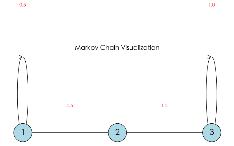
In the 3-state system above ($S=\{1, 2, 3\}$):
- State 1: 50% probability to stay ($1 \to 1$), 50% probability to jump to State 2 ($1 \to 2$).
- State 2: 100% probability to jump to State 3 ($2 \to 3$).
- State 3: 100% probability to stay ($3 \to 3$).
Where,
- State 1
- It can reach State 2 ($1 \to 2$).
- Transient. Although it has a 50% probability of staying temporarily, in the long run, it will definitely slip into State 2 eventually, and once it leaves, there is no way back.
- Inessential. Because State 2 cannot return to State 1, meaning there is a “point of no return”.
- State 2
- It can only reach State 3 ($2 \to 3$)
- Transient. It can only reach State 3, and once it leaves, there is no way back.
- Inessential. Because State 3 cannot return to State 2.
- State 3
- It can only reach itself.
- Recurrent, also Absorbing State.
- It can naturally return to itself, without “leaking” to any place of no return, so it is Essential.
Structural Properties
Irreducibility
In this chain, starting from any state, it is possible (in one or more steps) to reach any other state.
- Mathematical Symbol: For any $i, j \in S$, we have $i \leftrightarrow j$ (communicate).
- Intuition: The whole system is a cohesive unit, no isolated islands.
- Simple Understanding: If a city is called irreducible, it means the city is extremely navigable. No matter where you are (e.g., state $i$) and where you want to go (e.g., state $j$), you can always find a way (might need transfers, i.e., multiple steps, but you can get there).
Reducible: This means there are “traps” or “one-way areas” in the city. Once you enter a certain area, you can never go back to where you were. The system is divided into different “classes” or “parts”.
import networkx as nx
import matplotlib.pyplot as plt

def draw_chain(transitions, title, ax):
    G = nx.DiGraph()
    # Add edges and weights
    for u, v, p in transitions:
        G.add_edge(u, v, weight=p)

    # Use circular layout
    pos = nx.circular_layout(G)

    # Draw nodes
    nx.draw_networkx_nodes(G, pos, ax=ax, node_size=2000, node_color='lightblue', edgecolors='black')
    nx.draw_networkx_labels(G, pos, ax=ax, font_size=16, font_weight='bold')

    # Draw edges (with arc to avoid overlap)
    nx.draw_networkx_edges(G, pos, ax=ax, arrowstyle='->', arrowsize=25,
                           connectionstyle='arc3, rad=0.15')

    # Label probabilities
    edge_labels = {(u, v): f"{p}" for u, v, p in transitions}
    nx.draw_networkx_edge_labels(G, pos, edge_labels=edge_labels, ax=ax, label_pos=0.3, font_size=12)

    ax.set_title(title, fontsize=14)
    ax.axis('off')

# --- 1. Define Reducible Chain ---
# "3" here is a dead end (absorbing state), cannot return to "1" or "2"
transitions_reducible = [
    (1, 1, 0.5),
    (1, 2, 0.5),
    (2, 3, 1.0),
    (3, 3, 1.0)
]

# --- 2. Define Irreducible Chain ---
# We added 3->1, forming a closed loop, all states communicate
transitions_irreducible = [
    (1, 1, 0.5),
    (1, 2, 0.5),
    (2, 3, 1.0),
    (3, 1, 1.0)
]

# --- Plotting ---
fig, axes = plt.subplots(1, 2, figsize=(12, 5))

draw_chain(transitions_reducible, "Reducible (Broken Flow)", axes[0])
draw_chain(transitions_irreducible, "Irreducible (Connected Flow)", axes[1])

plt.tight_layout()
plt.show()
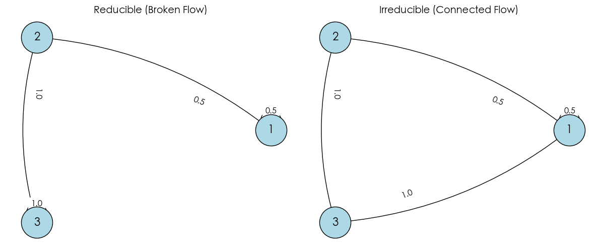
In the figures above:
- Left (Reducible): Contains a “trap” (State 3), once entered, cannot return to start.
- Right (Irreducible): The version we “surgically” fixed (added $3 \to 1$), all states communicate.
Periodicity
Periodicity describes the “rhythm” of the system returning to the original state. If it must take a fixed number of steps (e.g., even steps) to return home, then it is periodic.
Mathematical Definition: For state $i$, we collect all step numbers $n$ that allow the system to start from $i$ and return to $i$ (i.e., $p_{ii}^{(n)} > 0$) into a set:
$$ I_i = \{ n \ge 1 \mid p_{ii}^{(n)} > 0 \} $$The period $d(i)$ of state $i$ is defined as the Greatest Common Divisor (GCD) of all numbers in this set:
$$ d(i) = \text{gcd}(I_i) $$- Periodic: If $d(i) > 1$, state $i$ is called periodic.
- Here $d(i)$ is the period.
- Aperiodic: If $d(i) = 1$, state $i$ is called aperiodic.
- Meaning the GCD of the step set is 1.
- As long as state $i$ has a self-loop ($p_{ii} > 0$), it is aperiodic. This means you can come back in 1 step. Then $1$ is in set $I_i$. A set containing 1 must have a GCD of 1. So the state is aperiodic.
“Irreducible” can be “Periodic” or “Aperiodic”.
In an Irreducible Markov Chain, all states have the same period. That is, if one state in the chain is aperiodic, then the entire chain is aperiodic.
import networkx as nx
import matplotlib.pyplot as plt
def draw_subplot(transitions, title, ax, pos_type='circular'):
G = nx.DiGraph()
for u, v in transitions:
G.add_edge(u, v)
if pos_type == 'circular':
pos = nx.circular_layout(G)
else:
pos = nx.spring_layout(G, seed=42) # Fix seed for shape stability
# Draw nodes and edges
nx.draw_networkx_nodes(G, pos, ax=ax, node_size=800, node_color='lightgray', edgecolors='black')
nx.draw_networkx_labels(G, pos, ax=ax, font_size=12, font_weight='bold')
# Draw edges with arrows (use arc3 curve to avoid overlap)
nx.draw_networkx_edges(G, pos, ax=ax, arrowstyle='->', arrowsize=20,
connectionstyle='arc3, rad=0.1')
# Check self-loops, mark manually for visibility
self_loops = list(nx.selfloop_edges(G))
if self_loops:
nx.draw_networkx_edges(G, pos, ax=ax, edgelist=self_loops,
arrowstyle='->', arrowsize=20, connectionstyle='arc3, rad=0.5')
ax.set_title(title, fontsize=10)
ax.axis('off')
# --- Define 6 Cases ---
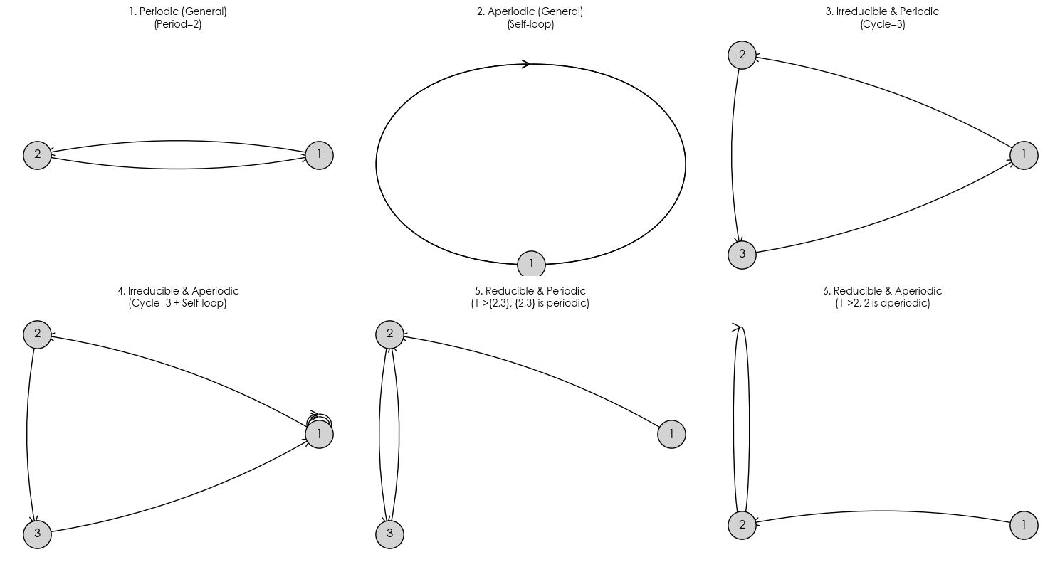
# 1. Simple Periodic
# Simplest back and forth, period 2
t_periodic = [(1, 2), (2, 1)]
# 2. Simple Aperiodic
# Self-loop breaks periodicity immediately, period 1
t_aperiodic = [(1, 1)]
# 3. Irreducible & Periodic
# A big loop, everyone communicates (irreducible), but steps must be multiple of 3
t_irr_per = [(1, 2), (2, 3), (3, 1)]
# 4. Irreducible & Aperiodic
# Communicates (irreducible), but added a self-loop at 1, rhythm broken (aperiodic)
t_irr_aper = [(1, 2), (2, 3), (3, 1), (1, 1)]
# 5. Reducible & Periodic
# 1 goes to 2 no return (reducible). 2 and 3 swap (period 2).
# Note: recurrent class {2,3} is periodic.
t_red_per = [(1, 2), (2, 3), (3, 2)]
# 6. Reducible & Aperiodic
# 1 goes to 2 no return (reducible). 2 has self-loop (aperiodic).
t_red_aper = [(1, 2), (2, 2)]
# --- Plotting ---
fig, axes = plt.subplots(2, 3, figsize=(15, 8))
axes = axes.flatten()
draw_subplot(t_periodic, "1. Periodic (General)\n(Period=2)", axes[0])
draw_subplot(t_aperiodic, "2. Aperiodic (General)\n(Self-loop)", axes[1])
draw_subplot(t_irr_per, "3. Irreducible & Periodic\n(Cycle=3)", axes[2])
draw_subplot(t_irr_aper, "4. Irreducible & Aperiodic\n(Cycle=3 + Self-loop)", axes[3])
draw_subplot(t_red_per, "5. Reducible & Periodic\n(1->{2,3}, {2,3} is periodic)", axes[4])
draw_subplot(t_red_aper, "6. Reducible & Aperiodic\n(1->2, 2 is aperiodic)", axes[5])
plt.tight_layout()
plt.show()
HIA Chain
HIA Chain is the “Gold Standard” in Markov Chains. It satisfies these three conditions simultaneously:
- H (Homogeneous): Transition rules $P$ never change.
- I (Irreducible): The whole system is connected, no dead ends.
- A (Aperiodic): No fixed cyclic rhythm.
Asymptotic Behavior of HIA Chains
Suppose
$$P = \begin{bmatrix} 0.7 & 0.3 \\ 0.4 & 0.6 \end{bmatrix}$$- Day 1 ($t=1, P^1$):$$\begin{bmatrix}
0.7 & 0.3 \\
0.4 & 0.6
\end{bmatrix}$$
- Large difference between two rows: Sunny today vs Rainy today affects tomorrow drastically.
- Day 5 ($t=5, P^5$):$$\begin{bmatrix}
0.5725 & 0.4275 \\
0.5700 & 0.4300
\end{bmatrix}$$
- Notice, the numbers in two rows start to look similar.
- Day 20 ($t=20, P^{20}$):$$\begin{bmatrix}
0.5714 & 0.4286 \\
0.5714 & 0.4286
\end{bmatrix}$$
- Here we see, initial weather 20 days ago has no influence on current prediction.
Limit Theorem for HIA Chains
For an HIA (Homogeneous, Irreducible, Aperiodic) Markov Chain, if its transition matrix is $P$, then as steps $n$ tend to infinity:
$$\lim_{n \to \infty} p_{ij}^{(n)} = \pi_j$$Here:
- $p_{ij}^{(n)}$: Probability of reaching state $j$ after $n$ steps starting from $i$.
- $\pi_j$: Steady state probability of state $j$ (constant, independent of starting state $i$).
Matrix form:
$$ \lim_{n \to \infty} P^n = \begin{bmatrix} \pi_0 & \pi_1 & \dots & \pi_k \ \pi_0 & \pi_1 & \dots & \pi_k \ \vdots & \vdots & \ddots & \vdots \ \pi_0 & \pi_1 & \dots & \pi_k \end{bmatrix} $$- Rows are identical: Every row in the final matrix is exactly the same.
- Every row is $\pi$: Each row is that unique steady state distribution vector $\pi = [\pi_0, \pi_1, \dots, \pi_k]$.
- Initial value forgotten: No matter you start from row 1 (state 0) or row $k$ (state $k$), your final probability of staying in a state is the same.
Stationary Distribution
Definition: A probability vector $\pi$, if
$$ \pi P = \pi, \quad \sum_i \pi_i = 1, \; \pi_i \geq 0 $$Then $\pi$ is called the Stationary Distribution of the Markov chain.
Significance: If the chain’s distribution is $\pi$ at some moment, it remains $\pi$ at any subsequent moment. It describes the Long-term State Distribution.
Mixing Time
Measure of convergence speed
Definition: Time required for the chain to get close to stationary distribution from initial distribution $\mu$.
Common Distance: Total Variation Distance
$$ d(t) = \max_\mu \| \mu P^t - \pi \|_{TV} $$Mixing Time: Smallest $t$ such that $d(t) \leq \epsilon$.
Ergodic Theorem
Theorem: For a finite Markov chain, if it is Irreducible and Aperiodic, then there exists a unique stationary distribution $\pi$, and:
$$ \lim_{n \to \infty} P(X_n = j \mid X_0 = i) = \pi_j \quad \forall i,j $$Also, time average converges to probability average:
$$ \frac{1}{N}\sum_{t=1}^N \mathbf{1}_{\{X_t=j\}} \to \pi_j $$Intuitive explanation: The proportion of time you stay in a state over the long term is exactly equal to the steady state probability of that state.
$$Time Average = Space Average$$This is invaluable in practice! It means we don’t need to solve complex equations to find $\pi$, just let the computer “run” a simulation (Monte Carlo), count how long it stays in each pit, and we can infer $\pi$.
Reversible Markov Chain
A Markov Chain $X = \{X_n\}$ is called a Reversible HIA Chain, if it satisfies all following conditions:
- Structural Condition (HIA). First, it must be an HIA chain, meaning:
- Homogeneous: Transition matrix $P$ constant.
- Irreducible: Any two states communicate.
- Aperiodic: Revisit steps have no fixed period (i.e., $\text{gcd}(I_i) = 1$).
- Reversibility Condition. The stationary distribution $\pi$ and transition matrix $P$ must satisfy Detailed Balance Equation: $$\pi_i P_{ij} = \pi_j P_{ji}, \quad \forall i, j \in S$$
Satisfying condition 1 guarantees the existence of a unique Stationary Distribution $\pi$.
Example
import numpy as np
import networkx as nx
import matplotlib.pyplot as plt
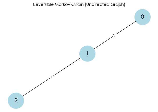
# 1. Define an Undirected Graph
# Weight here can be understood as "intimacy" or "channel width" between two states
G = nx.Graph()
G.add_edge(0, 1, weight=2)
G.add_edge(1, 2, weight=1)
# 2. Auto-build Transition Matrix P
# Rule: Prob of jumping from i to neighbor j = (weight of i,j) / (sum of all weights of i)
nodes = sorted(G.nodes())
n = len(nodes)
P = np.zeros((n, n))
for i in nodes:
total_weight = sum([G[i][nbr]['weight'] for nbr in G.neighbors(i)])
for j in G.neighbors(i):
P[i, j] = G[i][j]['weight'] / total_weight
print("--- Transition Matrix P ---")
print(P)
# 3. Compute Steady State pi
# Trick: For undirected graph, pi_i is proportional to "degree" of node i (sum of weights of connected edges)
degrees = [sum([G[i][nbr]['weight'] for nbr in G.neighbors(i)]) for i in nodes]
total_degree_sum = sum(degrees)
pi = np.array([d / total_degree_sum for d in degrees])
print("\n--- Steady State pi ---")
print(f"pi = {pi}")
# 4. Verify Detailed Balance: pi_i * P_ij = pi_j * P_ji ?
print("\n--- Flow Check ---")
# Check State 0 <-> State 1
flow_0_to_1 = pi[0] * P[0, 1]
flow_1_to_0 = pi[1] * P[1, 0]
print(f"Flow 0 -> 1: {pi[0]:.4f} * {P[0, 1]:.4f} = {flow_0_to_1:.4f}")
print(f"Flow 1 -> 0: {pi[1]:.4f} * {P[1, 0]:.4f} = {flow_1_to_0:.4f}")
if np.isclose(flow_0_to_1, flow_1_to_0):
print("✅ Detailed Balance satisfied between 0 and 1!")
else:
print("❌ Unbalanced")
# --- Plot ---
pos = nx.spring_layout(G, seed=42)
plt.figure(figsize=(6, 4))
nx.draw(G, pos, with_labels=True, node_color='lightblue', node_size=2000, font_size=16)
labels = nx.get_edge_attributes(G, 'weight')
nx.draw_networkx_edge_labels(G, pos, edge_labels=labels)
plt.title("Reversible Markov Chain (Undirected Graph)")
plt.show()
--- Transition Matrix P ---
[[0.         1.         0.        ]
 [0.66666667 0.         0.33333333]
 [0.         1.         0.        ]]

--- Steady State pi ---
pi = [0.33333333 0.5        0.16666667]

--- Flow Check ---
Flow 0 -> 1: 0.3333 * 1.0000 = 0.3333
Flow 1 -> 0: 0.5000 * 0.6667 = 0.3333
✅ Detailed Balance satisfied between 0 and 1!
Detailed Balance vs. Global Balance
Detailed Balance (Local) $\implies$ Global Balance. Proof:
Prove $\pi$ satisfies Global Balance Equation:
$$\sum_{i} \pi_i P_{ij} = \pi_j$$- Start: Look at LHS $\sum_{i} \pi_i P_{ij}$.
- Substitute: Use Detailed Balance ($\pi_i P_{ij} = \pi_j P_{ji}$), replace $\pi_i P_{ij}$ with $\pi_j P_{ji}$.$$\sum_{i} (\pi_j P_{ji})$$
- Extract: Pull constant $\pi_j$ out of summation.$$\pi_j \sum_{i} P_{ji}$$
- Normalize: Since $P$ is transition matrix, sum of probs from $j$ to all possible $i$ is 1 ($\sum_{i} P_{ji} = 1$).$$\pi_j \times 1 = \pi_j$$
- Conclusion: LHS equals RHS. Q.E.D.! ✅
Asymptotic Distribution of Reversible HIA Chains
“Asymptotic distribution of reversible HIA Chains” describes: As time tends to infinity, what state does a very special Markov chain stabilize into?
- HIA Chains: Acronym for Homogeneous, Irreducible, Aperiodic Markov Chains.
- Like a card shuffler that never changes rules, reaches all cards, and has no fixed rhythm.
- Key: HIA chain guarantees that no matter where you start, after sufficient time (asymptotic behavior, $n \to \infty$), the probability of system being in each state converges to a fixed value.
- Asymptotic Distribution: This “fixed value”. Limit of state distribution $\pi_n$ as $n \to \infty$.
- In HIA chains, this is the Stationary Distribution ($\pi$).
- Satisfies $\pi = \pi P$ (Global Balance).
- Reversibility: The “magic sauce”. If an HIA chain is reversible, its stationary distribution $\pi$ satisfies a stricter, simpler condition called Detailed Balance: $$\pi_i P_{ij} = \pi_j P_{ji}$$
- Means: At steady state, “flow” from $i$ to $j$ equals “flow” from $j$ back to $i$.
The so-called “Asymptotic distribution of reversible HIA Chains” is simply the unique stationary distribution $\pi$ derived using Detailed Balance equation ($\pi_i P_{ij} = \pi_j P_{ji}$).
Examples
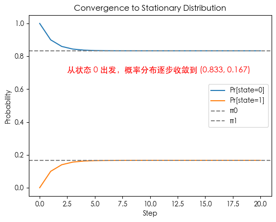
Example 1: Two-State Markov Chain
Simplest demo, clearly see convergence to stationary distribution.
Transition Matrix:
$$ P = \begin{bmatrix} 0.9 & 0.1 \\ 0.5 & 0.5 \end{bmatrix} $$(a) Stationary Distribution
Solve equation:
$$ \pi P = \pi $$i.e.:
$$ \pi_0 = 0.9\pi_0 + 0.5\pi_1 \quad\Rightarrow\quad 0.1\pi_0 = 0.5\pi_1 $$Combined with $\pi_0 + \pi_1 = 1$, we get:
$$ \pi = (0.833..., \; 0.166...) $$(b) Property Analysis
- Irreducible. Because two states are reachable from each other (both rows contain non-zero cross transitions).
- Aperiodic: Because $P_{00}>0, P_{11}>0$ (self-loops), can stay at original state → Period = 1
In summary, by Ergodic Theorem, this finite Markov chain is Ergodic, i.e., unique stationary distribution exists and converges to it from any initial value.
(c) Convergence Process
import numpy as np
import matplotlib.pyplot as plt

P = np.array([[0.9, 0.1],
              [0.5, 0.5]])

# Initial distribution
mu = np.array([1.0, 0.0])

distributions = [mu]
for _ in range(20):
    mu = mu @ P
    distributions.append(mu)

distributions = np.array(distributions)

plt.plot(distributions[:,0], label="Pr[state=0]")
plt.plot(distributions[:,1], label="Pr[state=1]")
plt.axhline(0.833, color="gray", linestyle="--", label="π0")
plt.axhline(0.167, color="gray", linestyle="--", label="π1")
plt.text(2.5, 0.7, "Start from state 0, prob distribution converges to (0.833, 0.167)", fontsize=12, color='red')
plt.xlabel("Step")
plt.ylabel("Probability")
plt.legend()
plt.title("Convergence to Stationary Distribution")
plt.show()
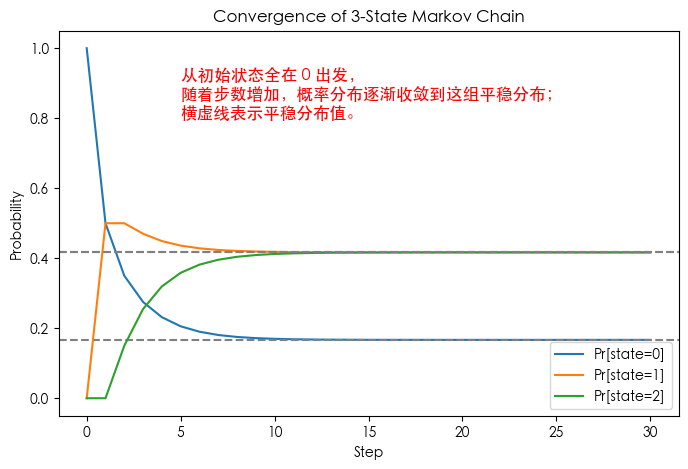
Example 2: Three-State Markov Chain
Demonstrates existence and uniqueness of stationary distribution in more complex chains.
Transition Matrix:
$$ P = \begin{bmatrix} 0.5 & 0.5 & 0.0 \\ 0.2 & 0.5 & 0.3 \\ 0.0 & 0.3 & 0.7 \end{bmatrix} $$- Irreducible: All states mutually reachable.
- Aperiodic: Self-loop prob $P_{ii} > 0$.
- Stationary Distribution: Solve $\pi P = \pi$, get unique $\pi$.
- Long-term Behavior: All initial distributions converge to $\pi$.
import numpy as np
import matplotlib.pyplot as plt

# 3-State Markov Chain Transition Matrix
P = np.array([[0.5, 0.5, 0.0],
              [0.2, 0.5, 0.3],
              [0.0, 0.3, 0.7]])

# Initial distribution (All in state 0)
mu = np.array([1.0, 0.0, 0.0])

# Calculate Stationary Distribution: Solve pi P = pi
eigvals, eigvecs = np.linalg.eig(P.T)
stat_dist = eigvecs[:, np.isclose(eigvals, 1)]
stat_dist = stat_dist[:,0]
stat_dist = stat_dist / stat_dist.sum()  # Normalize
print("Stationary distribution:", stat_dist.real)

# Iterative distribution evolution
distributions = [mu]
for _ in range(30):
    mu = mu @ P
    distributions.append(mu)

distributions = np.array(distributions)

# Plot
plt.figure(figsize=(8,5))
for i in range(3):
    plt.plot(distributions[:, i], label=f"Pr[state={i}]")
    plt.axhline(stat_dist[i].real, linestyle="--", color="gray")

plt.text(5, 0.8, "Start from all in 0,\nprob distribution converges to this stationary distribution;\nHorizontal dashed lines indicate stationary values.", fontsize=12, color='red')
plt.xlabel("Step")
plt.ylabel("Probability")
plt.title("Convergence of 3-State Markov Chain")
plt.legend()
plt.show()
Stationary distribution: [0.16666667 0.41666667 0.41666667]
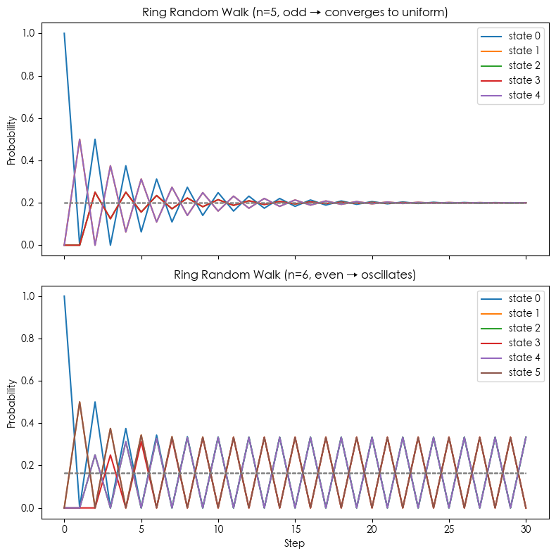
Example 3: Random Walk on a Cycle
Demonstrates effect of Periodicity on convergence.
States: $\{0,1,2,\dots,n-1\}$.
Transition Rule: From current $i$, move to $(i−1)\bmod n$ with prob 0.5, to $(i+1)\bmod n$ with prob 0.5. i.e.,
$$ P(i \to i+1 \bmod n) = 0.5, \quad P(i \to i-1 \bmod n) = 0.5 $$Irreducible: Can reach any state from any state.
Periodicity: If $n$ is even, Period=2; If $n$ is odd, Aperiodic.
Stationary Distribution: Uniform distribution $\pi_i = 1/n$.
Convergence:
- If $n$ odd → Chain is irreducible and aperiodic → Converges to uniform.
- If $n$ even → Chain has periodicity (Period=2) → Chain oscillates between “odd/even classes”, fails to converge to uniform.
import numpy as np
import matplotlib.pyplot as plt

def ring_rw_transition_matrix(n):
    """Generate n-state ring random walk transition matrix"""
    P = np.zeros((n, n))
    for i in range(n):
        P[i, (i-1)%n] = 0.5
        P[i, (i+1)%n] = 0.5
    return P

def simulate_chain(P, steps=30, start_state=0):
    """Compute distribution evolution from single point"""
    n = P.shape[0]
    mu = np.zeros(n)
    mu[start_state] = 1.0
    distributions = [mu]
    for _ in range(steps):
        mu = mu @ P
        distributions.append(mu)
    return np.array(distributions)

# Parameters
steps = 30
P5 = ring_rw_transition_matrix(5)
P6 = ring_rw_transition_matrix(6)

# Simulation
dist5 = simulate_chain(P5, steps)
dist6 = simulate_chain(P6, steps)

# Stationary distribution (Uniform for odd n; Even n doesn't have unique convergence)
pi5 = np.ones(5) / 5
pi6 = np.ones(6) / 6

# Plot
fig, axes = plt.subplots(2, 1, figsize=(8,8), sharex=True)

# n=5
for i in range(5):
    axes[0].plot(dist5[:, i], label=f"state {i}")
axes[0].hlines(pi5, 0, steps, colors="gray", linestyles="--", linewidth=1)
axes[0].set_title("Ring Random Walk (n=5, odd → converges to uniform)")
axes[0].set_ylabel("Probability")
axes[0].legend()

# n=6
for i in range(6):
    axes[1].plot(dist6[:, i], label=f"state {i}")
axes[1].hlines(pi6, 0, steps, colors="gray", linestyles="--", linewidth=1)
axes[1].set_title("Ring Random Walk (n=6, even → oscillates)")
axes[1].set_xlabel("Step")
axes[1].set_ylabel("Probability")
axes[1].legend()

plt.tight_layout()
plt.show()
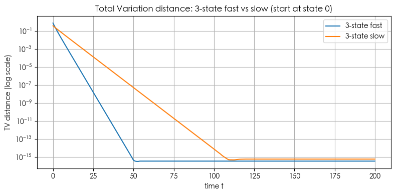
Example 4: Numerical Measure of Mixing Time (e.g. total variation distance convergence speed)
# Simulate Markov chains and compute total variation distance (TV) to the stationary distribution.
# We will:
# 1. Define several transition matrices (fast/slow 3-state, cycle random walks n=5 and n=6).
# 2. Compute TV distance over time starting from state 0.
# 3. Compute mixing times tau(epsilon) for epsilons = [0.1, 0.01, 0.001].
# 4. Plot TV vs time for comparisons and show a table of mixing times.
#
# Note: Plots use matplotlib (no seaborn) and each figure is a single plot as requested.
import numpy as np
import pandas as pd
import matplotlib.pyplot as plt
def stationary_from_P(P):
# solve pi = pi P with sum(pi)=1 -> transpose eigenvector of P^T for eigenvalue 1
w, v = np.linalg.eig(P.T)
idx = np.argmin(np.abs(w - 1.0))
pi = np.real(v[:, idx])
pi = pi / pi.sum()
pi = np.maximum(pi, 0)
pi = pi / pi.sum()
return pi
def tv_distance(p, q):
return 0.5 * np.sum(np.abs(p - q))
def tv_curve(P, p0, t_max):
n = P.shape[0]
pis = stationary_from_P(P)
p = p0.copy()
tvs = []
for t in range(t_max + 1):
tvs.append(tv_distance(p, pis))
p = p @ P
return np.array(tvs), pis
def mixing_time_from_tvs(tvs, eps):
# minimal t such that tvs[t] <= eps
below = np.where(tvs <= eps)[0]
return int(below[0]) if below.size > 0 else np.nan
# Define chains
# 3-state fast chain
P_fast = np.array([
[0.6, 0.3, 0.1],
[0.2, 0.6, 0.2],
[0.1, 0.3, 0.6]
])
# 3-state slow chain (more "sticky" on state 0)
P_slow = np.array([
[0.9, 0.08, 0.02],
[0.2, 0.7, 0.1],
[0.15, 0.15, 0.7]
])
# Cycle random walk
def cycle_P(n):
P = np.zeros((n, n))
for i in range(n):
P[i, (i+1) % n] = 0.5
P[i, (i-1) % n] = 0.5
return P
P_cycle5 = cycle_P(5)
P_cycle6 = cycle_P(6)
# initial distribution: start at state 0
def e0(n):
v = np.zeros(n); v[0]=1.0; return v
t_max = 200
# compute tv curves
tvs_fast, pi_fast = tv_curve(P_fast, e0(3), t_max)
tvs_slow, pi_slow = tv_curve(P_slow, e0(3), t_max)
tvs_c5, pi_c5 = tv_curve(P_cycle5, e0(5), t_max)
tvs_c6, pi_c6 = tv_curve(P_cycle6, e0(6), t_max)
# compute mixing times for selected epsilons
epsilons = [1e-1, 1e-2, 1e-3]
rows = []
for name, tvs in [
("3-state fast", tvs_fast),
("3-state slow", tvs_slow),
("cycle n=5", tvs_c5),
("cycle n=6", tvs_c6)
]:
entry = {"chain": name}
for eps in epsilons:
entry[f"tau({eps})"] = mixing_time_from_tvs(tvs, eps)
rows.append(entry)
df_mix = pd.DataFrame(rows)
# Plot 1: 3-state fast vs slow
plt.figure(figsize=(8,4))
plt.plot(tvs_fast, label='3-state fast')
plt.plot(tvs_slow, label='3-state slow')
plt.yscale('log') # show both fast and slow clearly on log scale
plt.xlabel('time t')
plt.ylabel('TV distance (log scale)')
plt.title('Total Variation distance: 3-state fast vs slow (start at state 0)')
plt.legend()
plt.grid(True)
plt.tight_layout()
plt.show()
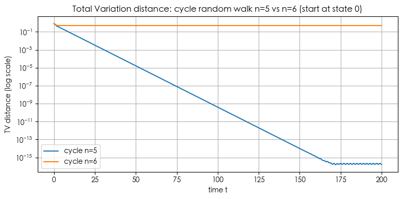
# Plot 2: cycle n=5 vs n=6
plt.figure(figsize=(8,4))
plt.plot(tvs_c5, label='cycle n=5')
plt.plot(tvs_c6, label='cycle n=6')
plt.yscale('log')
plt.xlabel('time t')
plt.ylabel('TV distance (log scale)')
plt.title('Total Variation distance: cycle random walk n=5 vs n=6 (start at state 0)')
plt.legend()
plt.grid(True)
plt.tight_layout()
plt.show()
# Also print stationary distributions for reference
pi_table = pd.DataFrame({
"chain": ["3-state fast", "3-state slow", "cycle n=5", "cycle n=6"],
"stationary": [pi_fast, pi_slow, pi_c5, pi_c6]
})
pi_table['stationary_str'] = pi_table['stationary'].apply(lambda x: np.array2string(x, precision=4, separator=', '))
pi_table = pi_table[['chain','stationary_str']]
display("Stationary distributions", pi_table)
'Stationary distributions'
| chain | stationary_str | |
|---|---|---|
| 0 | 3-state fast | [0.2857, 0.4286, 0.2857] |
| 1 | 3-state slow | [0.6466, 0.2328, 0.1207] |
| 2 | cycle n=5 | [0.2, 0.2, 0.2, 0.2, 0.2] |
| 3 | cycle n=6 | [0.1667, 0.1667, 0.1667, 0.1667, 0.1667, 0.1667] |
Scan to Share
微信扫一扫分享