Why Do We Need MCMC?
In short, because many distributions are only known in unnormalized forms, making traditional sampling/integration methods ineffective.
Goal: Sample from a complex distribution $\pi(x)$ (often only known as “unnormalized” $\tilde\pi(x)\propto \pi(x)$), or compute expectation/marginal:
$$ \mathbb{E}_\pi[f(X)] \;=\; \int f(x)\,\pi(x)\,dx. $$Reality Difficulties:
- High Dimensionality: As dimensions increase, grid/numerical integration explodes exponentially;
- Unknown Normalization Constant: In Bayesian context, the denominator $p(y)=\int p(y\mid \theta)p(\theta)\,d\theta$ in posterior $\pi(\theta\mid y)\propto p(y\mid \theta)p(\theta)$ is often intractable;
- Multi-modal/Strong Correlation: Variance of Rejection Sampling or Importance Sampling becomes huge or suffers from “weight degeneracy”.
Core Idea of Monte Carlo: Given samples $x^{(1)},\dots,x^{(T)}\sim \pi$, we can use sample mean
$$ \frac{1}{T}\sum_{t=1}^T f\!\big(x^{(t)}\big) $$to approximate $\mathbb{E}_\pi[f(X)]$. The problem is how to sample from $\pi$? This is exactly what MCMC solves: Without requiring the normalization constant, just being able to compute $\tilde\pi(x)$ (or its log), we can construct a stochastic process that “stays at $\pi$ in the long run” to draw samples.
Comparison with Other Approaches (Intuition):
- Variational Inference (VI): Fast, scalable, but approximates with a “tractable family”, introducing approximation bias;
- SMC/Particle Methods: Suitable for sequential problems, but design and resampling/annealing are complex;
- MCMC: Asymptotically Unbiased (can arbitrarily approximate $\pi$ if run long enough), but samples are correlated, computation can be expensive, and requires diagnostics/tuning.
Example
Suppose we want to sample from the following distribution:
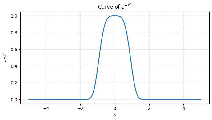
$$ \pi(x) \propto e^{-x^4}, \quad x \in \mathbb{R}. $$- This is a “super sharp” unimodal distribution.
- Normalization constant $Z=\int e^{-x^4}\,dx$ is unknown (cannot be solved by hand).
- Want to compute expectation $\mathbb{E}[X^2]$.
👉 Problem:
- Direct integration is impossible (analytically intractable).
- Rejection Sampling needs a “suitable envelope function”, but the tail here is very heavy, hard to find.
👉 Intuitive Conclusion: This is where MCMC shines: As long as we can compute $\tilde\pi(x)=e^{-x^4}$, i.e., the unnormalized density, we can design a Markov chain to converge to it.
# Plot e^{-x^4}
import numpy as np
import matplotlib.pyplot as plt
# Domain range (-5 to 5 is enough to see main shape)
x = np.linspace(-5, 5, 4001)
y = np.exp(-x**4)
plt.figure(figsize=(7, 4))
plt.plot(x, y, lw=2)
plt.title(r"Curve of $e^{-x^4}$")
plt.xlabel("x")
plt.ylabel(r"$e^{-x^4}$")
plt.grid(True, ls="--", alpha=0.4)
plt.tight_layout()
plt.show()
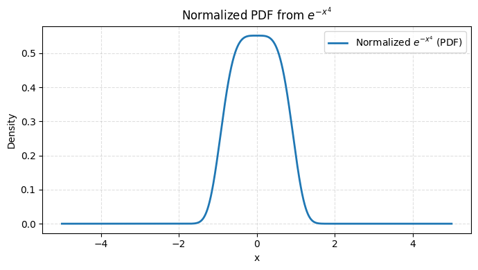
# Normalize e^{-x^4} to make it a Probability Density Function (PDF)
Z = np.trapezoid(y, x) # Numerical integration
pdf = y / Z
plt.figure(figsize=(7, 4))
plt.plot(x, pdf, lw=2, label="Normalized $e^{-x^4}$ (PDF)")
plt.title(r"Normalized PDF from $e^{-x^4}$")
plt.xlabel("x")
plt.ylabel("Density")
plt.grid(True, ls="--", alpha=0.4)
plt.legend()
plt.tight_layout()
plt.show()
From Markov Chain to Sampling
In short, by constructing a “correct Markov chain”, its stationary distribution becomes the target distribution; trajectory’s long-term distribution ≈ target distribution.
Turning Sampling into “Building a Chain”
Let state space be $\mathsf{X}$, want samples from target distribution $\pi$. We don’t sample directly, but construct a transition kernel $P(x,A)=\Pr(X_{t+1}\in A\mid X_t=x)$, making $\pi$ its Stationary Distribution (invariant):
$$ \pi(A) \;=\; \int_{\mathsf{X}} \pi(dx)\,P(x,A),\quad \forall A. $$Intuition: If you randomly pick a start point under $\pi$, then take a step according to $P$, the distribution remains unchanged. Such a “distribution-invariant” random walk, keeps walking, keeps staying on $\pi$.
Ensuring “Reachable, Aperiodic, Forgetting Start”
“Stationary” alone is not enough; we also need the chain to converge to $\pi$. Common sufficient conditions:
- Irreducible: Can reach any “mass” region from anywhere with positive probability in finite steps;
- Aperiodic: Not stuck in fixed cycles;
- Reasonable “Recurrence” (Harris recurrence etc. technical conditions).
With these, classic results tell us: regardless of initial distribution, as time $t\to\infty$, distribution $P^t(x_0,\cdot)$ converges to $\pi$ in Total Variation distance:
$$ \big\|P^t(x_0,\cdot)-\pi\big\|_{\mathrm{TV}}\to 0. $$So, discard early samples (burn-in), subsequent trajectory is approximately from $\pi$.
Why “Unnormalized is Fine”
Many MCMC constructions only need the ratio $\tilde\pi(x)\propto \pi(x)$. The reason lies in Detailed Balance / Reversibility (see next section): using only the ratio $\tilde\pi(y)/\tilde\pi(x)$ ensures “symmetric flow”, thereby getting $\pi$ as stationary distribution. No need for $Z$ is the key advantage of MCMC.
Example
To avoid introducing specific algorithms, determining let’s use the most familiar distribution: Uniform Distribution to illustrate.
Suppose target distribution is
$$ \pi(x) = \text{Uniform}\{1,2,3\}. $$We design a Markov chain:
- Walk among 3 states: 1, 2, 3;
- At each position, jump to another position with equal probability;
- E.g., at 1, jump to 2 with prob 0.5, to 3 with prob 0.5.
👉 The transition matrix P:
$$ P=\begin{bmatrix} 0 & 0.5 & 0.5 \\ 0.5 & 0 & 0.5 \\ 0.5 & 0.5 & 0 \end{bmatrix}. $$Let’s run it and see how its distribution evolves.
import numpy as np
import matplotlib.pyplot as plt

# Transition Matrix P
P = np.array([
    [0.0, 0.5, 0.5],
    [0.5, 0.0, 0.5],
    [0.5, 0.5, 0.0]
])

# Initial distribution: All in state 1
dist = np.array([1.0, 0.0, 0.0])
history = [dist]

# Evolve 20 steps
for t in range(20):
    dist = dist @ P
    history.append(dist)

history = np.array(history)

# Theoretical stationary distribution (Uniform)
pi = np.array([1/3, 1/3, 1/3])

# Plot
plt.figure(figsize=(6,4))
for i in range(3):
    plt.plot(history[:,i], label=f"State {i+1}")
plt.axhline(pi[0], color="k", linestyle="--", label="Stationary dist.")
plt.xlabel("Step")
plt.ylabel("Probability")
plt.title("Markov chain approaching uniform distribution")
plt.legend()
plt.show()
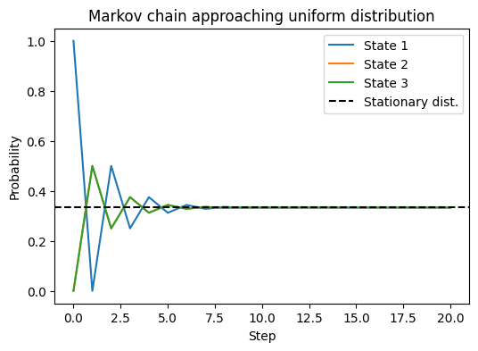
We can see:
- Initially distribution is all in state 1;
- As steps increase, three curves gradually approach $1/3$;
- Finally converges to stationary distribution (Uniform).
👉 Intuition: Markov chain’s “walking” allows us to sample from $\pi$ by relying on “long-term stay proportion” even if we don’t sample directly from $\pi$.
Theory and Intuition
Why it works, why it converges
In short,
- Stationary distribution exists, and satisfies detailed balance → Correctness.
- Convergence speed (Mixing time) affects sample quality.
- Smaller auto-correlation, larger ESS, “more efficient” chain.
Detailed Balance (Reversibility) and Stationarity
If there exists $\pi$ such that
$$ \pi(dx)\,P(x,dy) \;=\; \pi(dy)\,P(y,dx) \quad (\text{Symmetric Flow}) $$Then the chain is called reversible with respect to $\pi$, implying $\pi$ is a stationary distribution.
Intuition: Starting from $\pi$, the joint distribution of a forward step is same as a “backward step”, overall “no net flow”, so the steady state is “undisturbed”.
Many MCMC algorithms (MH, Gibbs, HMC, etc.) explicitly or implicitly construct this reversibility/invariance.
Convergence: Ergodic Theorem, LLN, CLT
When the chain is Ergodic (irreducible, aperiodic, and properly recurrent), we have:
Ergodic Theorem / Markov Chain Law of Large Numbers
$$ \frac{1}{T}\sum_{t=1}^T f(X_t) \;\xrightarrow{a.s.}\; \mathbb{E}_\pi[f(X)]. $$This guarantees using trajectory mean to estimate expectation is consistent.
Central Limit Theorem (CLT) (under geometric ergodicity etc. conditions)
$$ \sqrt{T}\Big(\bar f_T-\mathbb{E}_\pi[f]\Big)\ \Rightarrow\ \mathcal N\!\Big(0,\ \sigma_f^2\Big), $$Where
$$ \sigma_f^2 \;=\; \mathrm{Var}_\pi(f)\Big(1+2\sum_{k=1}^\infty \rho_k\Big), $$$\rho_k$ is the auto-correlation at lag $k$. Define Integrated Autocorrelation Time (IACT)
$$ \tau_{\text{int}} \;=\; 1+2\sum_{k\ge1}\rho_k, $$Then Effective Sample Size $\mathrm{ESS}\approx T/\tau_{\text{int}}$. Intuition: Stronger correlation (slow decay of $\rho_k$) means each sample has lower information, smaller ESS.
Mixing Time, Spectral Gap, and Geometric Convergence
Mixing Time characterizes approach speed of $P^t$ to $\pi$, commonly defined by TV distance:
$$ \tau(\varepsilon)\;=\;\min\{t:\ \sup_{x_0}\|P^t(x_0,\cdot)-\pi\|_{\mathrm{TV}}\le \varepsilon\}. $$For finite reversible chains, convergence speed is closely related to Spectral Gap $\gamma=1-\lambda_\star$ (second largest eigenvalue modulus $\lambda_\star$): $\tau(\varepsilon)$ typically scales as $\frac{1}{\gamma}\log(1/\varepsilon)$. Intuition: Large $\gamma$ ⇒ “Weak memory, fast forgetting”, faster mixing.
Conductance / Bottleneck characterizes “difficulty of crossing regions”, related to $\gamma$ via Cheeger inequality. Intuition: Multi-modal distribution, deep “valleys” between peaks ⇒ Small conductance ⇒ Slow mixing (easy to get “stuck in a mode”).
Burn-in, Thinning, Diagnostics (From Theory to Practice)
Burn-in: Early samples “not yet close to $\pi$” bias the estimate, discarding an initial segment is usually safer.
Thinning: “Subsampling” to save storage/reduce correlation, but from variance minimization perspective not strictly necessary; often better to keep all samples and use IACT/ESS for correct variance estimation.
Diagnostics (Intuition-driven):
- Trace: Wandering freely without obvious drift?
- ACF/ESS: Does correlation decay fast enough?
- Multi-chain R-hat: Do chains from multiple starting points mix together?
- Multi-modal: Any pattern of “stuck in mode” (long stay + sudden jump)?
Why MCMC can “Walk and Stay in High Density Areas”
View $\pi$ as Boltzmann distribution: $\pi(x)\propto e^{-U(x)}$, $U(x)=-\log \tilde\pi(x)$ looks like “energy landscape”. MCMC is like random thermal motion in the landscape:
- More willing to stay in Low Energy (High Density) regions;
- But through mechanisms like “perturbation/momentum/accept-reject”, still has chance to cross energy barriers to explore other regions;
- As long as mechanism guarantees invariant distribution is $\pi$ and chain is ergodic, long-term statistics will be correct.
Example
Let’s build a “Slow Mixing” chain:
- States $\{0,1\}$,
- From 0, stay with prob 0.95, jump to 1 with prob 0.05;
- From 1, same logic.
👉 Although its stationary distribution is still uniform $[0.5,0.5]$, “correlation” is very strong.
import numpy as np
import matplotlib.pyplot as plt

# Construct 2-state chain (Sticky)
P_slow = np.array([
    [0.95, 0.05],
    [0.05, 0.95]
])

# Simulate trajectory
T = 5000
x = np.zeros(T, dtype=int)
for t in range(1, T):
    x[t] = np.random.choice([0,1], p=P_slow[x[t-1]])

# Compute Auto-Correlation Function (ACF)
def autocorr(x, lag):
    n = len(x)
    x_mean = np.mean(x)
    num = np.sum((x[:n-lag]-x_mean)*(x[lag:]-x_mean)) # Auto-covariance
    den = np.sum((x-x_mean)**2) # Variance
    return num/den

lags = np.arange(50)
acfs = [autocorr(x, lag) for lag in lags]

# Plot
plt.figure(figsize=(6,4))
plt.bar(lags, acfs)
plt.xlabel("Lag")
plt.ylabel("Autocorrelation")
plt.title("ACF of slow-mixing 2-state chain")
plt.show()

Here you can see:
- Auto-Correlation Function (ACF) decays very slowly;
- Means adjacent samples are highly dependent, Effective Sample Size (ESS) is far less than total steps.
👉 Intuitive Summary:
- Markov chain will definitely converge to stationary distribution (if conditions met);
- But “Mixing Speed” varies: some equalize in few steps, some drag on;
- In MCMC, slow mixing chain has poor efficiency, resulting samples have “little information”.
Critical Indicators in Practice (No Algorithms Yet)
Only need $\tilde\pi(x)$: Can compute log-density up to constant, then MCMC is go.
Three things must be balanced:
- Invariance ($\pi$ is stationary) — if not invariant then long-term wrong;
- Reachable (Irreducible/Aperiodic) — if unreachable then pointless;
- Fast Mixing (Spectral gap/Conductance/Small IACT) — otherwise ESS too low, cost too high.
Error Assessment: Use IACT/ESS + Markov Chain CLT for MC variance and confidence intervals.
Multi-modal Warning: Multi-modal + high-dim correlation often leads to Metastability, need algorithms or strategies better at “climbing hills crossing valleys” (Tempering, Gradient methods, etc.) to improve conductance.
Summary
Purpose: Estimate expectation/sample from complex $\pi$; No normalization constant needed.
Method: Build a chain $P$ such that $\pi$ is invariant (often using Detailed Balance).
Condition: Irreducible + Aperiodic + Proper Recurrence ⇒ $P^t\to\pi$.
Assessment:
- Convergence (after burn-in) + Mixing (IACT/ESS, Spectral gap, Conductance)
- Diagnostics: Trace, ACF, R-hat, Multi-chain consistency
Error: $\mathrm{ESS}\approx T/\tau_{\text{int}}$, CLT gives confidence intervals.
Difficulty: Multi-modal/High-dim correlation ⇒ Slow mixing; Need better “moving strategies”.
Scan to Share
微信扫一扫分享