Deterministic Optimization
They are thought for convex function. If the function is not convex, we change to stochastic optimization.
| Algorithm | Category | Info Used | Geometric Intuition | Pros | Cons | MCMC Analog |
|---|---|---|---|---|---|---|
| Newton’s Method | 2nd Order | Gradient + Curvature (Hessian) | Parabolic Approximation (Bowl) | Convergence is extremely fast | Calculating $H^{-1}$ is too expensive | Similar to Langevin (Uses 2nd order) |
| Coordinate Descent | 0/1st Order | Single Variable Info | Move along axes | Simple, no full gradient needed | Slow convergence with strong correlation | Gibbs Sampling |
| Steepest Descent | 1st Order | Gradient | Steepest direction on tangent plane | Cheap computation, general | Prone to oscillation, slow convergence | Similar to HMC / MCMC |
Definition of Optimization Problem
Mathematically, a standard optimization problem is typically written in this “standard form”:
$$\begin{aligned} & \underset{x}{\text{minimize}} & & f(x) \\ & \text{subject to} & & g_i(x) \le 0, \quad i = 1, \dots, m \\ & & & h_j(x) = 0, \quad j = 1, \dots, p \end{aligned}$$Here are the three main characters:
- Decision Variable ($x$): The knobs we can control (e.g., model parameter weights).
- Objective Function ($f(x)$): Our metric. Usually minimizing “loss/cost” or maximizing “profit/likelihood”.
- Note: Maximizing $f(x)$ is equivalent to minimizing $-f(x)$, so we usually only study minimization.
- Constraints:
- Inequality Constraints ($g_i \le 0$): e.g., “Speed cannot exceed 100”.
- Equality Constraints ($h_j = 0$): e.g., “Energy must be conserved”.
Objective Function $f(x)$
To find the lowest point, this objective function $f(x)$ must follow three rules:
- Must be Scalar-Valued
- Requirement: Regardless of the dimension of input $x$ (e.g., you have 1 million parameters), the output of $f(x)$ must be a single real number (Scalar).
- Mathematical notation: $f: \mathbb{R}^n \to \mathbb{R}$
- Why?
- Because the core of optimization is “comparison”. We need to be able to say $f(x_1) < f(x_2)$. If $f(x)$ outputs a vector (e.g., two numbers “cost” and “time”), this becomes “multi-objective optimization”, which is another complex field. In standard optimization, you must synthesize them into one number (e.g., $0.5 \times \text{Cost} + 0.5 \times \text{Time}$).
- Must be Bounded Below
- This is to ensure “an optimal solution exists”.
- Requirement: The function cannot be a bottomless pit.
- Counter-example: $f(x) = x$ (domain is all real numbers).
- Want to minimize? I can pick $-100, -10000, -\infty \dots$
- You will never find the lowest point because there is no lowest point. The algorithm will run until memory overflow.
- Fix: Usually we require there exists a real number $M$ such that for all $x$, $f(x) \ge M$.
- Smoothness (for algorithms to run): If you want to use advanced algorithms like Newton’s method or Gradient Descent, the function $f(x)$ cannot look too arbitrary; it needs to satisfy continuity and differentiability.
- Continuity —— No broken roads
- Intuition: Walking on a mountain, the terrain cannot suddenly have “cliffs/fault lines”.
- Bad function: Step Function.
- e.g., $f(x)=1$ when $x < 0$, $f(x)=0$ when $x \ge 0$.
- This function is hard to optimize because at the break point, you don’t know where to step.
- Differentiability —— No sharp corners
- Intuition: This is the prerequisite for “Gradient Descent”.
- Gradient (derivative) represents slope. If the function has a sharp corner, the slope at that point is undefined (derivative does not exist).
- Bad function: $f(x) = |x|$ (Absolute value function).
- At the sharp point $x=0$, the derivative is undefined.
- Note: Although it is convex, standard gradient descent will fail here (needs Sub-gradient).
- Worse function: $f(x)$ is nowhere differentiable (like a jagged stock chart). This can only be hard-searched using “zero-order optimization” (algorithms that don’t look at gradients).
- Twice Differentiability —— For Newton’s Method
- If you want to use Newton’s method, the function not only needs slope (first derivative), but also “curvature” (second derivative).
- This means the terrain not only needs to be smooth, but the degree of bending must also vary smoothly, without sudden changes.
- Continuity —— No broken roads
Global vs. Local
- Global Optimum: The lowest point in the entire domain.
- Local Optimum: The lowest point within a small neighborhood, but there might be lower points outside.
Most deterministic algorithms (like Gradient Descent) can only guarantee finding a local optimum. Unless, the function has a special property —— Convexity.
Convex Function
Convex functions are the “good guys” in the optimization world. If your optimization problem is convex (Convex Optimization), then Local Optimum = Global Optimum. This is the property every optimization engineer dreams of.
Intuitive Definition
Imagine a bowl. If you pick any two points on the function graph and connect them with a line segment (chord), all points on this line segment are above (or coincide with) the function graph, then it is a convex function.
Mathematical Definition
A function $f: \mathbb{R}^n \to \mathbb{R}$ is convex if and only if for any $x, y$ and any $\theta \in [0, 1]$, the following is satisfied:
$$f(\theta x + (1-\theta)y) \le \theta f(x) + (1-\theta)f(y)$$- Left side $f(\dots)$: Represents the actual height at a point between $x$ and $y$.
- Right side $\dots f(\dots)$: Represents the height of the line connecting $x$ and $y$ (chord) at that point.
- $\le$: Means the actual height is always lower than or equal to the chord height.
Methods of Judgment
1D Case ($x$ is a real number): Check second derivative $f''(x)$. If for all $x$, $f''(x) \ge 0$, then it is a convex function.
- Example: $f(x) = x^2 \to f''(x) = 2 > 0$ (Convex).
- Example: $f(x) = -\log(x) \to f'(x) = -1/x \to f''(x) = 1/x^2 > 0$ (Convex).
Multi-dimensional Case ($x$ is a vector): Check Hessian Matrix ($\nabla^2 f(x)$). If for all $x$, the Hessian matrix is Positive Semidefinite (PSD) (i.e., all eigenvalues $\ge 0$), then it is a convex function.
Hessian Matrix
The Hessian matrix is a square matrix of second-order partial derivatives of a multivariate function. It describes the local curvature of the function.
Mathematical Definition: The “Full Form” of Second Derivatives
In high school math, for a single variable function $f(x)$:
- First derivative $f'(x)$: Slope.
- Second derivative $f''(x)$: Curvature (Concavity). $f''>0$ opens up, $f''<0$ opens down.
For a multivariate function $f(x_1, x_2, \dots, x_n)$, there isn’t just one second derivative, but a group. We need to consider the relationship between all pairs of variables. So we arrange them into an $n \times n$ matrix, which is the Hessian matrix $\mathbf{H}$ (or written as $\nabla^2 f(x)$):
$$\mathbf{H} = \begin{bmatrix} \frac{\partial^2 f}{\partial x_1^2} & \frac{\partial^2 f}{\partial x_1 \partial x_2} & \cdots & \frac{\partial^2 f}{\partial x_1 \partial x_n} \\ \frac{\partial^2 f}{\partial x_2 \partial x_1} & \frac{\partial^2 f}{\partial x_2^2} & \cdots & \frac{\partial^2 f}{\partial x_2 \partial x_n} \\ \vdots & \vdots & \ddots & \vdots \\ \frac{\partial^2 f}{\partial x_n \partial x_1} & \frac{\partial^2 f}{\partial x_n \partial x_2} & \cdots & \frac{\partial^2 f}{\partial x_n^2} \end{bmatrix}$$- Diagonal elements ($\frac{\partial^2 f}{\partial x_i^2}$): Represent the bending degree along the $i$-th coordinate axis.
- Off-diagonal elements ($\frac{\partial^2 f}{\partial x_i \partial x_j}$): Represent the “entanglement” degree between variable $i$ and variable $j$ (mixed partial derivatives). Usually, the matrix is symmetric (i.e., $H_{ij} = H_{ji}$).
The Hessian matrix tells us what the terrain under our feet looks like through its Eigenvalues. Now, imagine you are standing on a curved surface:
- Positive Definite Matrix (All eigenvalues > 0): Bowl bottom (Local Minimum)
- No matter which direction you go, the terrain curves upwards.
- This is a convex function (strictly convex).
- Negative Definite Matrix (All eigenvalues < 0): Mountain peak (Local Maximum)
- No matter which direction you go, the terrain curves downwards.
- Indefinite Matrix (Eigenvalues have both positive and negative): Saddle Point
- Going one direction is uphill (convex up), going another is downhill (concave down).
- Like a saddle, or a pass between two mountains. This is a headache in optimization because the gradient is also 0 here, easily fooling algorithms.
Positive Semidefinite (PSD)
You can analogize it to “non-negative numbers” ($\ge 0$) in real numbers. Just as we say a number is non-negative, saying a matrix is “positive semidefinite” means it is in some sense always “greater than or equal to zero”.
Core Definition
For an $n \times n$ real symmetric matrix $A$, if for any non-zero vector $x$ ($n$-dimensional column vector), we have:
$$x^T A x \ge 0$$Then we call matrix $A$ positive semidefinite. Here $x^T A x$ is called a Quadratic Form, which you can think of as an energy function or terrain height.
Take a $2 \times 2$ matrix as an example.
$$A = \begin{pmatrix} 2 & 0 \\ 0 & 1 \end{pmatrix}$$Geometric Intuition: What does it look like?
The quadratic form $x^T A x$ mentioned above is actually a function that maps vector $x$ to a real number. If we set vector $x = \begin{pmatrix} u \\ v \end{pmatrix}$, then:
$$x^T A x = \begin{pmatrix} u & v \end{pmatrix} \begin{pmatrix} 2 & 0 \\ 0 & 1 \end{pmatrix} \begin{pmatrix} u \\ v \end{pmatrix} = 2u^2 + 1v^2$$Plotting $z = 2u^2 + v^2$ in a 3D coordinate system, it is an Elliptic Paraboloid.
- Shape: Like a bowl curving up on both sides.
- Height: No matter what non-zero $(u, v)$ you pick, the calculated height $z$ is always positive. The lowest point is at the origin $(0,0)$, height 0.
- Conclusion: Since everywhere (except the origin) is higher than 0, this matrix is positive definite (and of course belongs to positive semidefinite).
Contrast: If one direction bends downwards (like a saddle surface), then it is not positive semidefinite.
Eigenvalue Judgment: What do the numbers say?
Without plotting, how do we know if the bowl opens upwards? This is where Eigenvalues come in.
For the diagonal matrix $A = \begin{pmatrix} 2 & 0 \\ 0 & 1 \end{pmatrix}$, its eigenvalues are right on the diagonal, very obvious:
- $\lambda_1 = 2$
- $\lambda_2 = 1$
Rule: All eigenvalues of a positive semidefinite matrix must be $\ge 0$. (If positive definite, eigenvalues must be strictly $> 0$).
So, why do eigenvalues determine the shape? Eigenvalues actually represent the bending degree of the paraboloid along the principal axes (i.e., curvature).
- $\lambda_1 = 2$: Indicates along the $u$ axis, the bowl wall is steeper (bends more, upwards).
- $\lambda_2 = 1$: Indicates along the $v$ axis, the bowl wall is slightly gentler (but also upwards).
As long as all directions “bend up” or are “flat” ($\ge 0$), the whole shape must be a “bowl” or “trough”, and won’t leak.
How to solve for eigenvalues of non-diagonal matrices
For non-diagonal matrices, we usually use the Characteristic Equation to solve for eigenvalues. The core idea starts from the definition of eigenvalues:
$$A\mathbf{v} = \lambda\mathbf{v}$$Here, $A$ is the matrix, $\mathbf{v}$ is a non-zero vector (eigenvector), and $\lambda$ is the eigenvalue we want to find. We can transform this equation into:
$$(A - \lambda I)\mathbf{v} = \mathbf{0}$$For this equation to have a non-zero solution (i.e., $\mathbf{v} \neq \mathbf{0}$), the determinant of the coefficient matrix $(A - \lambda I)$ must be zero. This gives us the general solution formula:
$$\det(A - \lambda I) = 0$$Here, $I$ is the Identity Matrix.
Example: Solving for eigenvalues of matrix $C = \begin{pmatrix} 1 & 2 \\ 2 & 1 \end{pmatrix}$.
- List the characteristic equation formula: $$\det(C - \lambda I) = 0$$
- Substitute the matrix: $$C - \lambda I = \begin{pmatrix} 1 & 2 \\ 2 & 1 \end{pmatrix} - \lambda \begin{pmatrix} 1 & 0 \\ 0 & 1 \end{pmatrix} = \begin{pmatrix} 1-\lambda & 2 \\ 2 & 1-\lambda \end{pmatrix}$$
- Calculate determinant for $2 \times 2$ matrix: $$\det(C - \lambda I) = (1-\lambda)(1-\lambda) - (2 \times 2)$$
- Expand and simplify: $$(1 - 2\lambda + \lambda^2) - 4 = 0$$ $$\lambda^2 - 2\lambda - 3 = 0$$ This is the characteristic polynomial.
- Solve quadratic equation: $(\lambda - 3)(\lambda + 1) = 0$
- Result: $\lambda_1 = 3, \lambda_2 = -1$.
Conclusion: Eigenvalues of matrix $C$ are 3 and -1.
import numpy as np
import matplotlib.pyplot as plt

# 1. Set x and y grid range
x = np.linspace(-3, 3, 50)
y = np.linspace(-3, 3, 50)
X, Y = np.meshgrid(x, y)

# 2. Define two quadratic form functions
# Case 1: Positive Definite Matrix A = [[2, 0], [0, 1]]
# z = 2x^2 + 1y^2
Z_positive = 2 * X**2 + 1 * Y**2

# Case 2: Indefinite Matrix B = [[1, 0], [0, -3]]
# z = 1x^2 - 3y^2
Z_indefinite = 1 * X**2 - 3 * Y**2

# 3. Create plot
fig = plt.figure(figsize=(14, 6))

# --- Plot 1 (Bowl) ---
ax1 = fig.add_subplot(1, 2, 1, projection='3d')
ax1.plot_surface(X, Y, Z_positive, cmap='viridis', alpha=0.8, edgecolor='none')
ax1.set_title('Positive Definite (Bowl)\nEigenvalues: 2, 1')
ax1.set_xlabel('X axis')
ax1.set_ylabel('Y axis')
ax1.set_zlabel('Z value')
ax1.scatter(0, 0, 0, color='red', s=50, label='Global Min') # Mark min

# --- Plot 2 (Saddle) ---
ax2 = fig.add_subplot(1, 2, 2, projection='3d')
ax2.plot_surface(X, Y, Z_indefinite, cmap='coolwarm', alpha=0.8, edgecolor='none')
ax2.set_title('Indefinite (Saddle)\nEigenvalues: 1, -3')
ax2.set_xlabel('X axis')
ax2.set_ylabel('Y axis')
ax2.set_zlabel('Z value')
ax2.scatter(0, 0, 0, color='green', s=50, label='Saddle Point') # Mark saddle

plt.tight_layout()
plt.show()
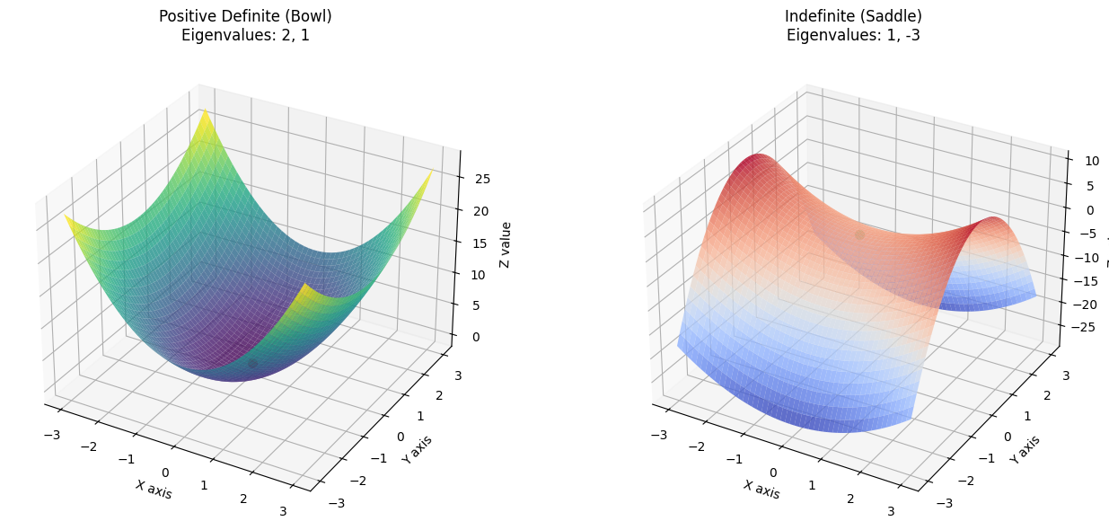
Notice the origin $(0,0)$ in the image above:
- In the Left Image (Bowl), if you place a small ball anywhere, it will eventually roll down to the red lowest point.
- In the Right Image (Saddle), if you walk along the $X$ axis, it’s uphill; but if you walk along the $Y$ axis, it’s downhill.
Newton’s Method
Suitable for 1D
Newton’s method is a Second-Order Optimization Algorithm.
- First-order algorithms (like Gradient Descent): Only use gradient (slope) information, telling us which way to go to decrease the function value.
- Second-order algorithms (like Newton’s Method): Use not only gradient, but also second derivative (curvature) information. It knows not only how steep the slope is, but also how much the slope bends.
Core Idea: Quadratic Approximation
The core logic of Newton’s method is: Fit a quadratic function (parabola/paraboloid) to the curve at the current position, and then jump directly to the lowest point of this paraboloid.
Step 1: Second-Order Taylor Expansion (Fitting)
Near the current point $x_k$, we expand the complex objective function $f(x)$ into a quadratic polynomial:
$$f(x) \approx f(x_k) + \nabla f(x_k)^T (x - x_k) + \frac{1}{2} (x - x_k)^T \mathbf{H}(x_k) (x - x_k)$$- The first part is a plane (gradient).
- The second part is bending (Hessian matrix).
Step 2: Take Derivative to Find Extremum (Jump)
We want to find the lowest point of this approximate paraboloid. Simple, take the derivative of the above expression and set it to 0:
$$\nabla f(x_k) + \mathbf{H}(x_k)(x - x_k) = 0$$Step 3: Derive Update Formula
Solve the above equation for $x$, which is the next point $x_{k+1}$ we want to go to:
$$\mathbf{x}_{k+1} = \mathbf{x}_k - \mathbf{H}^{-1}(x_k) \nabla f(x_k)$$This is Newton’s iterative formula. See, it multiplies by an extra $\mathbf{H}^{-1}$ (inverse of Hessian matrix) compared to Gradient Descent.
Stopping Criteria
Gradient Judgment: Is the slope flat?
- Theoretically the hardest standard. Necessary condition for optimum is gradient being 0.
- Criterion: Stop when gradient norm is less than a threshold (e.g., $10^{-6}$).
- Formula: $||\nabla f(x_k)|| < \epsilon$
- Intuition: If the ground under your feet is as flat as an airport (almost no slope), you are likely at the bottom.
Step Size Judgment: Still moving?
- Sometimes gradient calculation is expensive, or terrain is very flat, we can check change in $x$.
- Criterion: If update step $x_{k+1}$ and previous step $x_k$ almost overlap.
- Formula: $||x_{k+1} - x_k|| < \epsilon$
- Intuition: If one step only advances 0.000001 mm, not much point continuing.
Function Value Judgment: Is gain still significant?
- From a “cost-benefit” perspective.
- Criterion: Objective function value $f(x)$ almost stops decreasing.
- Formula: $|f(x_{k+1}) - f(x_k)| < \epsilon$
- Intuition: If after much effort, cost only drops by 1 cent, call it a day (Diminishing returns).
Budget Judgment (Mandatory): Time up?
- Prevent infinite loops or timeout.
- Criterion: Reach Max Iterations.
- Intuition: Boss only gave 1000 bucks (compute resource), stop when money runs out regardless of result.
Pros & Cons
- ✅ Extremely fast convergence: Usually reaches bottom in a few steps (Quadratic convergence speed).
- ❌ High computational cost: Calculating inverse of Hessian $\mathbf{H}$ takes $O(n^3)$. Almost unusable in high dimensions ($n$ is large). Thus, generally used for 1D problems.
- ❌ Sensitive to initial value: If start point is too far from optimum and function is non-convex, Newton’s method might fly off to space.
Examples
Example 1: Manual Calculation
Objective: $f(x) = x^2 - 4x + 4$ (Parabola opening up, min clearly at $x=2$).
Assume we start far away at $x_0 = 10$.
- Calc Gradient (1st deriv): $g(x) = f'(x) = 2x - 4$. At $x_0=10$, $g(10) = 16$.
- Calc Hessian (2nd deriv): $h(x) = f''(x) = 2$. Constant $2$ (Standard quadratic function).
- Newton Update: $x_{new} = x_{old} - \frac{g(x)}{h(x)}$ –> $x_1 = 10 - \frac{16}{2} = 2$.
- Check if $x=2$ is optimal:
- Gradient Check: $f'(2) = 2(2) - 4 = 0$. ✅ Slope is 0.
- Hessian Check: $f''(2) = 2 > 0$. ✅ Minimum.
- Try “One More Step”: $x_{new} = 2 - 0/2 = 2$. ✅ Algorithm stays put.
Result: Surprise? Just one step, jumped from $10$ directly to $2$ (Global Optimum).
Example 2
This example lets you intuitively feel the power of Newton’s Method, especially its quadratic convergence and stopping criteria. A non-quadratic function is chosen:
$$f(x, y) = x^4 + y^4$$import numpy as np
import matplotlib.pyplot as plt
# --- 1. Define objective, gradient, hessian ---
# Objective: f(x, y) = x^4 + y^4 (Min at 0,0)
def func(p):
x, y = p
return x**4 + y**4
# Gradient: [4x^3, 4y^3]
def gradient(p):
x, y = p
return np.array([4 * x**3, 4 * y**3])
# Hessian: [[12x^2, 0], [0, 12y^2]]
def hessian(p):
x, y = p
return np.array([[12 * x**2, 0],
[0, 12 * y**2]])
# --- 2. Newton's Method Core ---
def newton_optimization(start_point, tolerance=1e-6, max_iter=100):
path = [start_point]
x = np.array(start_point, dtype=float)
print(f"{'Iter':<5} | {'x':<20} | {'Grad Norm':<15}")
print("-" * 45)
for i in range(max_iter):
g = gradient(x)
H = hessian(x)
# --- Stop Criterion 1: Gradient small enough? ---
grad_norm = np.linalg.norm(g)
print(f"{i:<5} | {str(x):<20} | {grad_norm:.8f}")
if grad_norm < tolerance:
print(f"\n✅ Trigger Stop: Grad Norm {grad_norm:.2e} < {tolerance}")
break
# --- Newton Update ---
# Formula: x_new = x - H^-1 * g
# Tip: Don't use inv(), utilize solve() for stability
try:
step = np.linalg.solve(H, g)
except np.linalg.LinAlgError:
print("⚠️ Hessian singular, stop.")
break
x = x - step
path.append(x)
return np.array(path)
# --- 3. Run ---
start_pos = [2.0, 2.5] # Start from (2, 2.5)
path_newton = newton_optimization(start_pos)
# --- 4. Visualize ---
x_grid = np.linspace(-3, 3, 100)
y_grid = np.linspace(-3, 3, 100)
X, Y = np.meshgrid(x_grid, y_grid)
Z = X**4 + Y**4
plt.figure(figsize=(8, 7))
plt.contour(X, Y, Z, levels=30, cmap='gray_r', alpha=0.4) # Contours
plt.plot(path_newton[:, 0], path_newton[:, 1], 'o-', color='red', lw=2, label="Newton's Path")
# Mark start/end
plt.scatter(path_newton[0,0], path_newton[0,1], color='blue', s=100, label='Start')
plt.scatter(path_newton[-1,0], path_newton[-1,1], color='green', marker='*', s=200, zorder=5, label='Converged')
plt.title(f"Newton's Method Optimization on $f(x,y) = x^4 + y^4$")
plt.legend()
plt.grid(True, linestyle='--')
plt.show()
Iter  | x                    | Grad Norm
---------------------------------------------
0     | [2.  2.5]            | 70.21573898
1     | [1.33333333 1.66666667] | 20.80466340
2     | [0.88888889 1.11111111] | 6.16434471
3     | [0.59259259 0.74074074] | 1.82647251
4     | [0.39506173 0.49382716] | 0.54117704
5     | [0.26337449 0.32921811] | 0.16034875
6     | [0.17558299 0.21947874] | 0.04751074
7     | [0.11705533 0.14631916] | 0.01407726
8     | [0.07803688 0.09754611] | 0.00417104
9     | [0.05202459 0.06503074] | 0.00123586
10    | [0.03468306 0.04335382] | 0.00036618
11    | [0.02312204 0.02890255] | 0.00010850
12    | [0.01541469 0.01926837] | 0.00003215
13    | [0.01027646 0.01284558] | 0.00000953
14    | [0.00685097 0.00856372] | 0.00000282
15    | [0.00456732 0.00570915] | 0.00000084

✅ Trigger Stop: Grad Norm 8.36e-07 < 1e-06
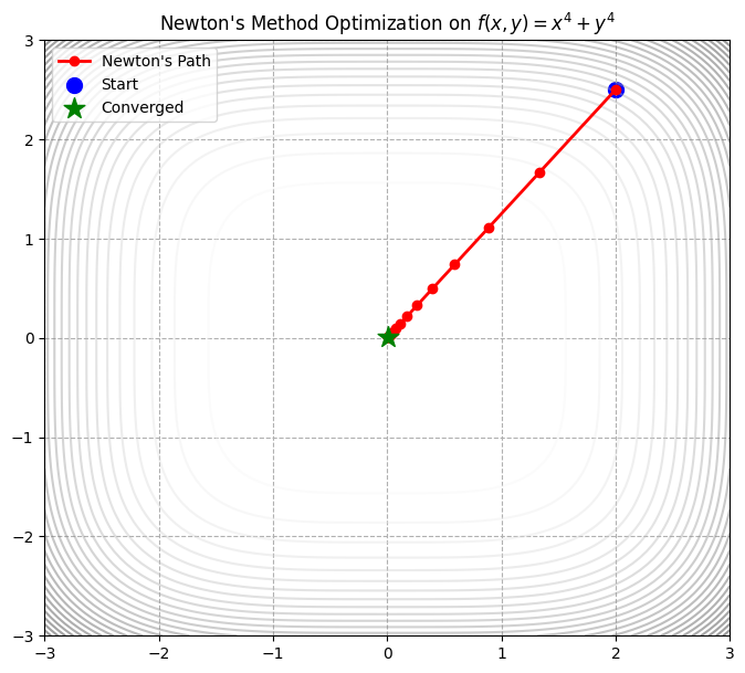
Code Highlights
- Convergence Speed: Observe Grad Norm. Once near the bottom, gradient norm drops precipitously (e.g., from 0.1 to 0.0001). Characteristic of quadratic convergence.
np.linalg.solve(H, g): Do not useinv(). Solving linear equations is faster and more stable.- Stopping Criteria: Hard threshold
grad_norm < tolerance.
Coordinate Descent (Simple Relaxation)
Suitable for N dim
In continuous optimization context, this usually refers to Coordinate Descent, or Gauss-Seidel method in linear equations. This is actually the deterministic version of Gibbs Sampling!
Coordinate Descent is a “Divide and Conquer” strategy.
- Newton/Gradient Descent: “All-in attack”. All variables $(x_1, \dots, x_n)$ move together.
- Coordinate Descent (Relaxation): “Single soldier combat”. Only one variable moves at a time, others fixed.
Geometric Intuition: Walking in Manhattan. Can only move East-West (X-axis) or North-South (Y-axis). To reach the lowest point, move East, stop, move South, repeat.
Algorithm Flow
Minimize $f(x_1, \dots, x_n)$.
- Init: Pick $x^{(0)}$.
- Loop (until converge):
- Update $x_1$: Fix $x_2, \dots, x_n$, find $x_1$ minimizing $f$.
$$x_1^{(new)} = \underset{x_1}{\text{argmin}} \ f(x_1, x_2^{(old)}, \dots, x_n^{(old)})$$
- $f$ becomes 1D function, use derivatives to solve min.
- Update $x_2$: Fix $x_1^{(new)}, x_3, \dots, x_n$, find $x_2$.
- …
- Update $x_n$: Fix previous, find $x_n$.
- Update $x_1$: Fix $x_2, \dots, x_n$, find $x_1$ minimizing $f$.
$$x_1^{(new)} = \underset{x_1}{\text{argmin}} \ f(x_1, x_2^{(old)}, \dots, x_n^{(old)})$$
Core Logic: Solve one 1D optimization problem at a time.
Pros & Cons
Pros
- No Gradient: If single variable optimization is easy (analytic solution), no gradient needed.
- Manhattan Move: Zig-zag trajectory along axes.
- Applicability: Great for low coupling variables, or L1 regularization (Lasso).
Cons
- Very slow with strong correlation. Imagine a narrow diagonal valley (variables $x$ and $y$ highly correlated, e.g., $f=(x-y)^2$). Coordinate descent struggles, hitting walls, advancing tiny bits.
Examples
Basic Example
Objective: $f(x, y) = x^2 + xy + y^2$. 1D bowl, but $xy$ term makes contours slanted ellipses.
Manual Derivation:
- Optimize $x$: Fix $y$. $d/dx = 2x + y = 0 \implies x = -y/2$.
- Optimize $y$: Fix $x$. $d/dy = x + 2y = 0 \implies y = -x/2$.
import numpy as np
import matplotlib.pyplot as plt

# Objective: f(x,y) = x^2 + xy + y^2
def func(p):
    x, y = p
    return x**2 + x*y + y**2

# --- Coordinate Descent ---
def coordinate_descent(start_point, n_cycles=10):
    path = [start_point]
    x, y = start_point

    print(f"{'Step':<5} | {'x':<10} | {'y':<10} | {'Action'}")
    print("-" * 45)

    for i in range(n_cycles):
        # 1. Fix y, optimize x
        x_new = -y / 2
        path.append([x_new, y])
        print(f"{i*2+1:<5} | {x_new:<10.4f} | {y:<10.4f} | Update x")
        x = x_new

        # 2. Fix x, optimize y
        y_new = -x / 2
        path.append([x, y_new])
        print(f"{i*2+2:<5} | {x:<10.4f} | {y_new:<10.4f} | Update y")
        y = y_new

    return np.array(path)

# --- Run ---
start_pos = [2.0, 2.0]
path_cd = coordinate_descent(start_pos, n_cycles=5)

# --- Visualize ---
x_grid = np.linspace(-2.5, 2.5, 100)
y_grid = np.linspace(-2.5, 2.5, 100)
X, Y = np.meshgrid(x_grid, y_grid)
Z = X**2 + X*Y + Y**2

plt.figure(figsize=(8, 7))
plt.contour(X, Y, Z, levels=20, cmap='viridis', alpha=0.5)

# Plot zig-zag path
plt.plot(path_cd[:, 0], path_cd[:, 1], 'o-', color='red', lw=2, label="Coordinate Descent Path")
plt.scatter(0, 0, marker='*', s=200, color='gold', zorder=5, label="Global Min")

plt.title("Simple Relaxation (Coordinate Descent) on $x^2 + xy + y^2$")
plt.legend()
plt.grid(True, linestyle='--')
plt.show()
Step  | x          | y          | Action
---------------------------------------------
1     | -1.0000    | 2.0000     | Update x
2     | -1.0000    | 0.5000     | Update y
3     | -0.2500    | 0.5000     | Update x
4     | -0.2500    | 0.1250     | Update y
5     | -0.0625    | 0.1250     | Update x
6     | -0.0625    | 0.0312     | Update y
7     | -0.0156    | 0.0312     | Update x
8     | -0.0156    | 0.0078     | Update y
9     | -0.0039    | 0.0078     | Update x
10    | -0.0039    | 0.0020     | Update y
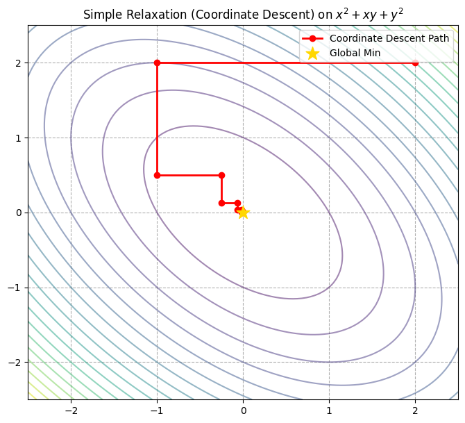
Image Analysis:
- Right angle turns: Path completely horizontal/vertical. Manhattan distance.
- Convergence: Slowly spirals in due to $x, y$ coupling.
- Contrast: Newton’s method would jump to $(0,0)$ in one step.
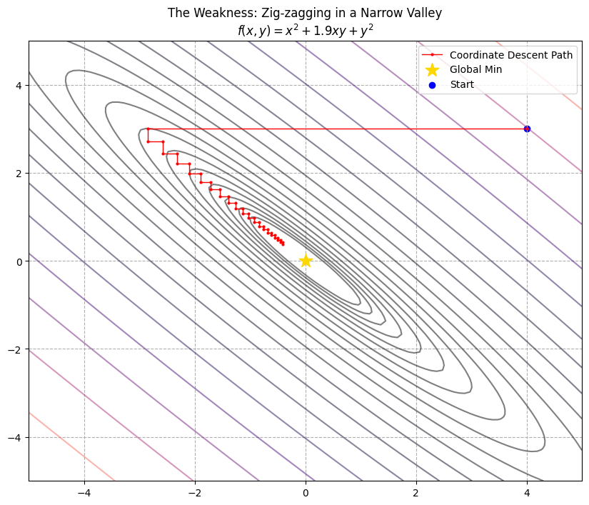
Example: Extremely Slow with Strong Correlation
Scenario: The Narrow Diagonal Valley
Terrain is a very narrow, slanted valley.
- Bottom is a diagonal line ($y \approx -x$).
- To descend, must adjust both $x$ and $y$.
Coordinate Descent is OCD, only moves one coordinate.
- Wants to go left-down, moves left, hits wall.
- Stops, moves down, hits wall.
- Bounces between walls, tiny steps, running in place.
Mathematical Construction Change coupling coefficient from 1 to 1.9. $f(x, y) = x^2 + \mathbf{1.9}xy + y^2$.
- Update: $x = -0.95y$, $y = -0.95x$.
- Values shrink by only 5% each iteration. Extremely slow.
import numpy as np
import matplotlib.pyplot as plt

# Pathological function, high coupling
def func(p):
    x, y = p
    # 1.9 coefficient makes ellipse extremely narrow
    return x**2 + 1.9 * x * y + y**2

# --- Coordinate Descent ---
def coordinate_descent_bad_case(start_point, n_cycles=10):
    path = [start_point]
    x, y = start_point

    for i in range(n_cycles):
        # 1. Update x: 2x + 1.9y = 0 => x = -0.95y
        x = -0.95 * y
        path.append([x, y])

        # 2. Update y: 1.9x + 2y = 0 => y = -0.95x
        y = -0.95 * x
        path.append([x, y])

    return np.array(path)

# --- Run Contrast ---
start_pos = [4.0, 3.0]
# Run 20 cycles
path_cd = coordinate_descent_bad_case(start_pos, n_cycles=20)

# --- Visualize ---
x_grid = np.linspace(-5, 5, 100)
y_grid = np.linspace(-5, 5, 100)
X, Y = np.meshgrid(x_grid, y_grid)
Z = X**2 + 1.9*X*Y + Y**2

plt.figure(figsize=(10, 8))
plt.contour(X, Y, Z, levels=np.logspace(-1, 2, 20), cmap='magma', alpha=0.5)

# Plot path
plt.plot(path_cd[:, 0], path_cd[:, 1], '.-', color='red', lw=1, markersize=4, label="Coordinate Descent Path")
plt.scatter(0, 0, marker='*', s=200, color='gold', zorder=5, label="Global Min")
plt.scatter(start_pos[0], start_pos[1], color='blue', label='Start')

plt.title("The Weakness: Zig-zagging in a Narrow Valley\n$f(x,y) = x^2 + 1.9xy + y^2$")
plt.legend()
plt.grid(True, linestyle='--')
plt.show()

print(f"Start: {start_pos}")
print(f"End (after 40 steps): {path_cd[-1]}")
print(f"True Min: [0, 0]")
Start: [4.0, 3.0]
End (after 40 steps): [-0.40582786  0.38553647]
True Min: [0, 0]
Analysis:
- “Sewing Machine” Effect: Path is dense red zigzag lines.
- Running in Place: After 40 steps, still far from origin. Previous example took 5 cycles.
- Intuition: Moving a wide sofa through a narrow corridor. Gradient Descent tilts the sofa. Coordinate Descent moves left 1cm, hits wall, down 1cm, hits wall.
Steepest Descent
Suitable for N dim
Steepest Descent is a First-Order Optimization Algorithm.
- Intuition: Blindfolded on a mountain. To get down fast, feel around with feet, step in direction of steepest downward slope.
- Math Core:
- Gradient ($\nabla f$): Steepest uphill.
- Negative Gradient ($-\nabla f$): Steepest downhill.
- Contrast:
- Unlike Coordinate Descent, can move any direction.
- Unlike Newton’s, is “myopic”, only sees slope under feet.
Core Idea: Greedy Downhill
Core formula:
$$x_{k+1} = x_k - \alpha \nabla f(x_k)$$Two key roles:
- Direction ($\nabla f(x_k)$): Where to go.
- Step Size ($\alpha$, Learning Rate): How big a step.
In classical definition, $\alpha$ is determined by Line Search. In modern ML, often a fixed hyperparameter.
Choice of Step Size $\alpha$ (Line Search)
Strict “Steepest Descent” uses Line Search:
$$\alpha_k = \underset{\alpha > 0}{\text{argmin}} \ f(x_k - \alpha \nabla f(x_k))$$Determine direction, walk to lowest point in that direction, then change direction.
Pros & Cons
- Low cost: Fast gradient calculation.
- Path shape: Vertical Zig-zag.
- Convergence: Linear.
- Weakness: Sensitive to step size & oscillation in valleys.
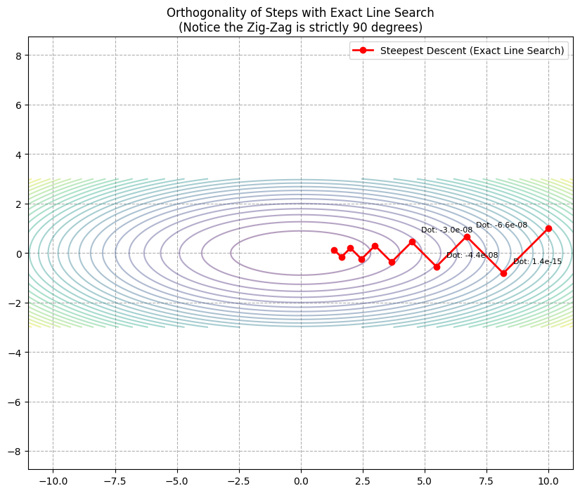
Zig-Zagging
Famous weakness. Adjacent steps are orthogonal (perpindicular) with Exact Line Search. In narrow valleys, bounces between walls, oscillating wildly. Reasons for Momentum.
Examples
Basic Example
Using the narrow valley function $f(x, y) = x^2 + 10y^2$. $y$ slope is 10x steeper.
import numpy as np
import matplotlib.pyplot as plt

# Objective: f(x,y) = x^2 + 10y^2
def func(p):
    x, y = p
    return x**2 + 10 * y**2

# Gradient: [2x, 20y]
def gradient(p):
    x, y = p
    return np.array([2 * x, 20 * y])

# --- Steepest Descent ---
def steepest_descent(start_point, learning_rate, n_iter=20):
    path = [start_point]
    p = np.array(start_point)

    for _ in range(n_iter):
        grad = gradient(p)
        p = p - learning_rate * grad
        path.append(p)

    return np.array(path)

# --- Run ---
start_pos = [8.0, 2.0]

# 1. Moderate LR (0.05)
path_good = steepest_descent(start_pos, learning_rate=0.05, n_iter=20)

# 2. Large LR (0.09) - Near oscillation
path_oscillate = steepest_descent(start_pos, learning_rate=0.09, n_iter=20)

# --- Visualize ---
x_grid = np.linspace(-10, 10, 100)
y_grid = np.linspace(-4, 4, 100)
X, Y = np.meshgrid(x_grid, y_grid)
Z = X**2 + 10*Y**2

plt.figure(figsize=(12, 6))

# Left: Normal LR
plt.subplot(1, 2, 1)
plt.contour(X, Y, Z, levels=20, cmap='viridis', alpha=0.5)
plt.plot(path_good[:, 0], path_good[:, 1], 'o-', color='blue', label='LR=0.05')
plt.title("Good Learning Rate\n(Steady Descent)")
plt.legend()
plt.grid(True, linestyle='--')

# Right: Oscillating LR
plt.subplot(1, 2, 2)
plt.contour(X, Y, Z, levels=20, cmap='viridis', alpha=0.5)
plt.plot(path_oscillate[:, 0], path_oscillate[:, 1], 'o-', color='red', label='LR=0.09')
plt.title("Large Learning Rate\n(Zig-zag / Oscillation)")
plt.legend()
plt.grid(True, linestyle='--')

plt.show()
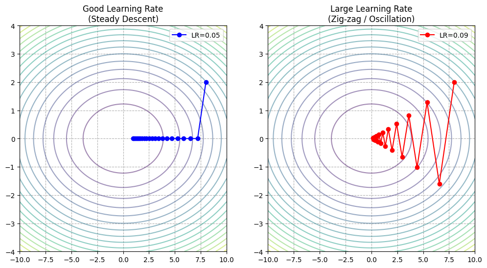
- Left (Good LR): Curved path, steady approach. Not straight line to center.
- Right (Large LR - Oscillation): Jumping crazily in $y$ direction (Steep). Wasting energy bouncing between North/South walls while slowly advancing East/West.
Example: Exact Line Search
Orthogonal steps.
import numpy as np
import matplotlib.pyplot as plt
from scipy.optimize import minimize_scalar

def func(p):
    x, y = p
    return x**2 + 10 * y**2

def gradient(p):
    x, y = p
    return np.array([2 * x, 20 * y])

# --- Steepest Descent w/ Exact Line Search ---
def steepest_descent_exact_line_search(start_point, n_iter=10):
    path = [start_point]
    x_k = np.array(start_point)

    for _ in range(n_iter):
        grad = gradient(x_k)

        # Define 1D function for alpha
        def line_obj(alpha):
            return func(x_k - alpha * grad)

        # Find best alpha
        res = minimize_scalar(line_obj)
        best_alpha = res.x

        x_new = x_k - best_alpha * grad
        path.append(x_new)

        if np.linalg.norm(x_new - x_k) < 1e-6:
            break
        x_k = x_new

    return np.array(path)

# --- Run ---
start_pos = [10.0, 1.0]
path_exact = steepest_descent_exact_line_search(start_pos, n_iter=10)

# --- Visualize ---
x_grid = np.linspace(-11, 11, 100)
y_grid = np.linspace(-3, 3, 100)
X, Y = np.meshgrid(x_grid, y_grid)
Z = X**2 + 10*Y**2

plt.figure(figsize=(10, 8))
plt.contour(X, Y, Z, levels=30, cmap='viridis', alpha=0.4)

plt.plot(path_exact[:, 0], path_exact[:, 1], 'o-', color='red', lw=2, label='Steepest Descent (Exact Line Search)')

# Annotate Right Angles
for i in range(len(path_exact)-2):
    p1 = path_exact[i]
    p2 = path_exact[i+1]
    p3 = path_exact[i+2]

    v1 = p2 - p1
    v2 = p3 - p2

    dot_product = np.dot(v1, v2)
    if i < 4:
        plt.annotate(f"Dot: {dot_product:.1e}", xy=p2, xytext=(10, 10), textcoords='offset points', fontsize=8)

plt.title("Orthogonality of Steps with Exact Line Search\n(Notice the Zig-Zag is strictly 90 degrees)")
plt.axis('equal')
plt.legend()
plt.grid(True, linestyle='--')
plt.show()
Example: The Grand Showdown
Three algorithms in one arena. Terrain: Skewed & Coupled:
$$f(x, y) = x^2 + 1.5xy + 2y^2$$Analysis: Elliptical bowl, slanted ($1.5xy$ term).
- Coordinate Descent: Nightmare (no slanted moves).
- Steepest Descent: Challenge (oscillation).
- Newton’s Method: Piece of cake (Quadratic surface).
import numpy as np
import matplotlib.pyplot as plt

# --- 1. Arena ---
# f(x, y) = x^2 + 1.5xy + 2y^2
def func(p):
    x, y = p
    return x**2 + 1.5*x*y + 2*y**2

def gradient(p):
    x, y = p
    return np.array([2*x + 1.5*y, 1.5*x + 4*y])

def hessian(p):
    return np.array([[2, 1.5],
                     [1.5, 4]])

# --- 2. Player 1: Steepest Descent ---
def steepest_descent(start, lr=0.15, steps=20):
    path = [start]
    x = np.array(start)
    for _ in range(steps):
        grad = gradient(x)
        x = x - lr * grad
        path.append(x)
    return np.array(path)

# --- 3. Player 2: Coordinate Descent ---
def coordinate_descent(start, steps=10):
    path = [start]
    x, y = start
    for _ in range(steps):
        # Opt x: d/dx = 2x + 1.5y = 0 -> x = -0.75y
        x = -0.75 * y
        path.append([x, y])

        # Opt y: d/dy = 1.5x + 4y = 0 -> y = -0.375x
        y = -0.375 * x
        path.append([x, y])
    return np.array(path)

# --- 4. Player 3: Newton's Method ---
def newton_method(start, steps=5):
    path = [start]
    x = np.array(start)
    H = hessian(x)
    H_inv = np.linalg.inv(H)

    for _ in range(steps):
        grad = gradient(x)
        x = x - H_inv @ grad
        path.append(x)
        if np.linalg.norm(grad) < 1e-6: break
    return np.array(path)

# --- 5. Visuals ---
start_pos = [8.0, -6.0]

path_sd = steepest_descent(start_pos)
path_cd = coordinate_descent(start_pos)
path_newton = newton_method(start_pos)

x_grid = np.linspace(-9, 9, 100)
y_grid = np.linspace(-9, 9, 100)
X, Y = np.meshgrid(x_grid, y_grid)
Z = X**2 + 1.5*X*Y + 2*Y**2

plt.figure(figsize=(10, 9))
plt.contour(X, Y, Z, levels=30, cmap='gray_r', alpha=0.3)

plt.plot(path_sd[:,0], path_sd[:,1], 'o-', color='red', label='Steepest Descent (Gradient)')
plt.plot(path_cd[:,0], path_cd[:,1], '.-', color='orange', label='Coordinate Descent (Staircase)')
plt.plot(path_newton[:,0], path_newton[:,1], 'x--', color='blue', lw=2, markersize=12, label="Newton's Method (Direct)")

plt.scatter(start_pos[0], start_pos[1], color='black', s=100, label='Start')
plt.scatter(0, 0, marker='*', s=300, color='gold', zorder=10, label='Global Min')

plt.title("Deterministic Optimization Showdown\n$f(x,y) = x^2 + 1.5xy + 2y^2$")
plt.legend()
plt.axis('equal')
plt.grid(True, linestyle='--')
plt.show()
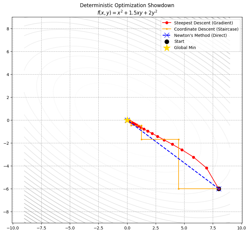
Comparison:
- Newton’s Method (Blue): 1 step to bullseye. “God mode” with curvature info.
- Steepest Descent (Red): Curved path, steady approach. Good cost-performance.
- Coordinate Descent (Orange): Staircase. Struggles with coupling. Least efficient here.
Scan to Share
微信扫一扫分享