Bayesian Image Segmentation in Practice

Taking image segmentation as a case study.

The Cornerstone of Bayesian Image Segmentation: The Game Between Likelihood and Prior

In computer vision, the goal of Image Segmentation is to assign a label (e.g., foreground or background) to every pixel in an image. Here, we denote the observed image as $Y$ ($y_{ij} \in \mathbb{R}$) and the target labels (Mask) as $L$ ($l_{ij} \in \{1, 2\}$).

From a Bayesian perspective, we are looking for the Posterior Probability, which is the probability of the true labels $L$ given the observed image $Y$.

According to Bayes’ theorem, the Posterior Probability can be written as:

Replacing variables with ours:

This formula breaks down an extremely difficult problem into two separately solvable parts:

1. Likelihood $P(Y|L)$: If the true labels are really $L$, what is the probability of generating the noisy image $Y$ we see?
2. Prior $P(L)$: Before seeing the image, based on common sense, what should the labels $L$ look like?

Our ultimate goal is to find an $L$ that maximizes the product of likelihood and prior, which is the MAP (Maximum A Posteriori) estimate.

Python Example: Building Our “Test Field”

Before exploring how to solve this, we must first create the “observed data” and “ground truth” labels using code.

Assume the training samples follow Gaussian distributions: $y_{ij} | l_{ij}=1 \sim N[\mu_1, \sigma_1^2]$ and $y_{ij} | l_{ij}=2 \sim N[\mu_2, \sigma_2^2]$

The following code generates our Ground Truth and the observed image with Gaussian noise.

import numpy as np
import matplotlib.pyplot as plt

# ==========================================
# 1. Simulate Real World (Ground Truth)
# ==========================================
# Assume a 50x50 image
rows, cols = 50, 50
true_L = np.ones((rows, cols)) # Label 1 for background
# Draw a square in the center as foreground (Label 2)
true_L[15:35, 15:35] = 2

# ==========================================
# 2. Simulate Observation Process (Likelihood Generation)
# ==========================================
# We know color distribution parameters for different labels from training samples (mean mu and variance sigma)
# Background (Label 1) is darker, Foreground (Label 2) is brighter
mu_1, sigma_1 = 0.0, 1.0  
mu_2, sigma_2 = 3.0, 1.0  

# Generate observed image Y by adding Gaussian noise based on true labels
Y = np.zeros_like(true_L, dtype=float)
# Assign N(mu_1, sigma_1) color values to pixels labeled 1
Y[true_L == 1] = np.random.normal(mu_1, sigma_1, np.sum(true_L == 1))
# Assign N(mu_2, sigma_2) color values to pixels labeled 2
Y[true_L == 2] = np.random.normal(mu_2, sigma_2, np.sum(true_L == 2))

# ==========================================
# 3. Visualize Our Generated Data
# ==========================================
fig, axes = plt.subplots(1, 2, figsize=(10, 5))

axes[0].imshow(true_L, cmap='gray')
axes[0].set_title("Ground Truth Mask (L)\nLabel 1(Black), Label 2(White)")
axes[0].axis('off')

axes[1].imshow(Y, cmap='viridis')
axes[1].set_title("Noisy Observation (Y)\nWhat the computer sees")
axes[1].axis('off')

plt.tight_layout()
plt.show()

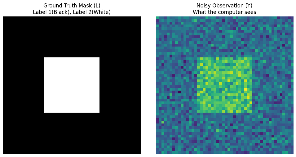
You can see the perfect black and white square on the left (God’s perspective $L$), and the noisy colorful image on the right (Mortal’s perspective $Y$). The task now is: Given only the right image $Y$ and Gaussian parameters, how can the computer deduce the left image $L$?

Traditional Classification — The Disaster of Assuming “Absolute Independence”

Before introducing Bayesian MRF, it is necessary to see how “predecessors” did it and why they failed. This will help us appreciate the greatness of MRF.

The Traditional Method makes a fatal assumption in image processing: Absolute Independence.

It assumes that each pixel’s label $l_i$ is on its own, completely unrelated to its neighbors:

The Logic of “Cleaning Only One’s Own Doorstep”

Because of the absolute independence assumption, the prior probability $P(L)$ becomes a constant or completely ineffective. When classifying, the computer only looks at the color of the current pixel (The classification only considers itself).

Its logic is very simple and crude:

1. Look at the current pixel value $y_{ij}$.
2. Calculate the Gaussian probability $P(y_{ij}|l_{ij}=1)$ that it belongs to Label 1 (background).
3. Calculate the Gaussian probability $P(y_{ij}|l_{ij}=2)$ that it belongs to Label 2 (foreground).
4. Whichever probability is higher, assign that class. (This is pure Maximum Likelihood Estimation, MLE)

Python Example: Implementing Traditional Classification and Witnessing the “Disaster”

We continue from the observed data Y generated in the previous section and implement this traditional method with a few lines of code.

# ==========================================
# Continue from variables: Y, mu_1, sigma_1, mu_2, sigma_2
# ==========================================

# Use likelihood calculation directly
L_traditional = np.ones_like(Y)

# 1. Calculate likelihood for Label 1 (Background)
# Based on Normal Distribution N(mu_1, sigma_1^2)
likelihood_1 = np.exp(-0.5 * ((Y - mu_1) / sigma_1)**2) / sigma_1

# 2. Calculate likelihood for Label 2 (Foreground)
# Based on Normal Distribution N(mu_2, sigma_2^2)
likelihood_2 = np.exp(-0.5 * ((Y - mu_2) / sigma_2)**2) / sigma_2

# 3. Simple comparison: if likelihood for foreground is greater, set label to 2
L_traditional[likelihood_2 > likelihood_1] = 2

# ==========================================
# Visualize the Disaster Result
# ==========================================
fig, axes = plt.subplots(1, 3, figsize=(12, 4))

axes[0].imshow(true_L, cmap='gray')
axes[0].set_title("Ground Truth")
axes[0].axis('off')

axes[1].imshow(Y, cmap='viridis')
axes[1].set_title("Noisy Observation (Y)")
axes[1].axis('off')

axes[2].imshow(L_traditional, cmap='gray')
axes[2].set_title("Traditional Method\n(Noisy & Isolated pixels)")
axes[2].axis('off')

plt.tight_layout()
plt.show()

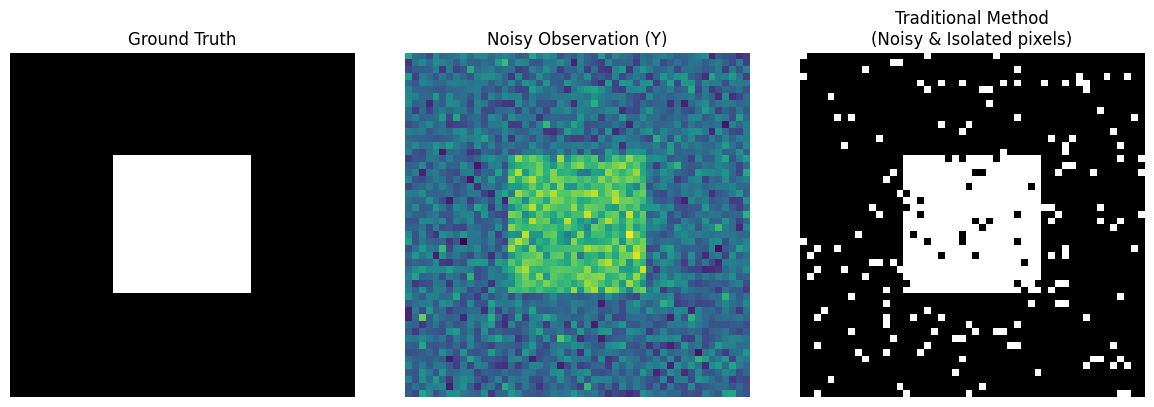
Notice the third image above (Traditional Method): Although it barely makes out the outline of a square, the inside is full of black “pockmarks,” and the outside background is full of white “snowflakes.”

Why does this happen?

Because Gaussian noise causes some background pixel values to suddenly become very high. The traditional method “sees the trees but misses the forest”; seeing a high value, it immediately misclassifies it as foreground. It lacks the common sense that “the physical world is continuous; if a white dot is surrounded by black dots, it is most likely noise.”

Bayesian MRF Method — Introducing “Spatial Common Sense” (Modeling the Homogeneity)

The results above tell us that for image segmentation, one absolutely cannot “only look at oneself.” The real physical world is continuous: if a pixel is foreground, its surrounding pixels are likely foreground too.

Therefore, we “Not Assume independency anymore”! We use Bayesian methods combined with MRF to teach “spatial common sense” to the computer.

Likelihood Function: Still Each to Their Own

In the Bayesian formula $P(L|Y) \propto P(Y|L) P(L)$, for the first part, the likelihood function $P(Y|L)$, we still maintain the independence assumption: the process of generating image colors is generated independently by each pixel under a Gaussian distribution.

Evolution of Prior Probability: Modeling the Homogeneity

The magic happens in the second part, the prior probability $P(L)$. Since pixel labels are no longer independent, how do we mathematically describe that “they are close together”?

A brilliant solution: Define it as a Gibbs Distribution!

The core here is Gibbs Energy $E(L)$. We design a penalty mechanism:

• If my neighbor and I have the same label (homogeneous), the energy is low, and the system is happy.
• If my neighbor and I have different labels (heterogeneous), the system applies a “penalty for diff”.

Using the concept of “Clique” defined by neighbors, we can write this penalty formula:

Here $\alpha$ is a crucial hyperparameter representing “how strong you want the homogeneity”. The larger $\alpha$ is, the less the computer dares to label a pixel differently from its surroundings.

The Final Form of Posterior Probability

Now, multiplying likelihood and prior, we get this ultimate formula:

This formula looks long, but if you take its negative log (-log), it turns into a very elegant “energy minimization” problem.

For any pixel $i$, calculating the total energy for taking a certain label $l_i$:

Total Energy = Data Term (Likelihood) + Smoothness Term (Prior)

Python Example: Creating the “Total Energy” Detector

To prepare for the optimization in the next section, we first need to write this “energy calculation” function. This is the soul detector of MRF.

# ==========================================
# Variables from previous sections: 
# Y (Observed Image)
# mu_1, sigma_1 (Gaussian params for Label 1 Background)
# mu_2, sigma_2 (Gaussian params for Label 2 Foreground)
# ==========================================

def get_pixel_energy(padded_L, Y, r, c, label_candidate, alpha):
    """
    Calculate the total Gibbs Energy for point (r, c) assuming label_candidate
    padded_L: Currently padded label map (for neighbor access)
    """
    # 1. Data Term (from Likelihood)
    # After -log: (y - mu)^2 / (2*sigma^2) + log(sigma)
    y_val = Y[r-1, c-1]
    
    if label_candidate == 1:
        energy_data = 0.5 * ((y_val - mu_1) / sigma_1)**2 + np.log(sigma_1)
    else:
        energy_data = 0.5 * ((y_val - mu_2) / sigma_2)**2 + np.log(sigma_2)
        
    # 2. Smoothness Term (from Prior MRF)
    # Formula: alpha * sum(|l_i - l_j|)
    # Find neighbors (up, down, left, right)
    neighbors = [padded_L[r-1, c], padded_L[r+1, c], 
                 padded_L[r, c-1], padded_L[r, c+1]]
                 
    # Calculate difference penalty with neighbors
    energy_smooth = alpha * sum([abs(label_candidate - n) for n in neighbors])
    
    # 3. Return Total Energy (Lower energy means more likely label)
    return energy_data + energy_smooth

# Let's test a point
# Add padding to traditional result for testing
padded_L_test = np.pad(L_traditional, 1, mode='edge')

# Test energy for point (25, 25) being Label 1 and Label 2 (Assume alpha=1.2)
e1 = get_pixel_energy(padded_L_test, Y, 25, 25, label_candidate=1, alpha=1.2)
e2 = get_pixel_energy(padded_L_test, Y, 25, 25, label_candidate=2, alpha=1.2)

print(f"Energy for (25, 25) being Background (1): {e1:.2f}")
print(f"Energy for (25, 25) being Foreground (2): {e2:.2f}")
print("Conclusion: System prefers the label with lower energy!")

Energy for (25, 25) being Background (1): 7.23
Energy for (25, 25) being Foreground (2): 1.25
Conclusion: System prefers the label with lower energy!

The Ultimate Weapons for Finding MAP — Simulated Annealing & Gibbs Sampling

In the previous section, we successfully wrote the calculation formula for “Total Energy.” Lower total system energy means higher posterior probability, and thus a more perfect image segmentation result.

However, for an image, even if each pixel only has two labels (1 or 2), there are $2^{2500}$ possible combinations! We cannot exhaustively enumerate all label combinations to find the one with the lowest energy.

So, how do we find the optimal solution in this astronomical solution space?

Simulated Annealing (SA) combined with Gibbs Sampler.

Inner Engine: Gibbs Sampler

If we try to update all pixels at once, the system will crash. The core wisdom of Gibbs Sampling is: Update only one pixel at a time, pretending all other pixels are fixed.

And thanks to the Markov property of MRF, when updating the current pixel, we “only look at neighbors”.

1. Calculate energy $E_1$ if current pixel becomes Label 1.
2. Calculate energy $E_2$ if current pixel becomes Label 2.
3. Use Gibbs formula to convert energy to probability, then roll the dice to decide its label.

Outer Commander: Simulated Annealing (SA)

To prevent Gibbs Sampling from getting stuck in local dead ends (e.g., stuck on a stubborn noise pixel), we introduce “Temperature $T$”. “The S.A. requires a sampling done by a Gibbs Sampler”.

• High Temperature: The system is very active. Even if a label increases energy (worse), it has a probability of being accepted. This allows the algorithm to jump out of “pockmark” traps.
• Cooling Phase: As iterations progress, the system gradually “cools down,” becoming more inclined to accept only labels that lower energy (better). Finally, it freezes in the perfect MAP state.

Python Example: Witnessing the Miracle!

Now, we assemble all the code blocks. We initialize a starting point $L_0$, then start this powerful Bayesian MRF engine!

# ==========================================
# Variables from previous: 
# true_L (Ground Truth), Y (Noisy Image), L_traditional (Traditional Result)
# get_pixel_energy() function
# ==========================================

def mrf_bayesian_segmentation(Y, initial_L, alpha=1.2, iter_max=15, T_init=3.0, T_end=0.1):
    """
    Use Simulated Annealing + Gibbs Sampling to find MAP for Image Segmentation
    """
    rows, cols = Y.shape
    
    # 1. Initialize Start (Init L0) 
    # To speed up convergence, start from traditional method result instead of random guess
    L = np.copy(initial_L) 
    
    # Calculate geometric cooling rate
    tau = -np.log(T_end / T_init) / (iter_max - 1)
    
    print("🚀 Starting Bayesian MRF Optimization Engine...")
    
    # Outer Loop: Simulated Annealing (SA)
    for it in range(iter_max):
        T = T_init * np.exp(-tau * it) # Current Temperature
        
        # Pad image for neighbor handling
        padded_L = np.pad(L, 1, mode='edge')
        
        # Inner Loop: Gibbs Sampler scans whole image
        for r in range(1, rows + 1):
            for c in range(1, cols + 1):
                
                # Calculate local total energy for Label 1 and Label 2
                E_1 = get_pixel_energy(padded_L, Y, r, c, label_candidate=1, alpha=alpha)
                E_2 = get_pixel_energy(padded_L, Y, r, c, label_candidate=2, alpha=alpha)
                
                # Convert energy difference to probability using Gibbs formula
                # P(L=1) = exp(-E_1/T) / (exp(-E_1/T) + exp(-E_2/T))
                # Simplify to Logistic form to prevent overflow:
                prob_1 = 1.0 / (1.0 + np.exp((E_1 - E_2) / T))
                
                # Roll the dice! (Sample based on probability)
                if np.random.rand() < prob_1:
                    padded_L[r, c] = 1
                else:
                    padded_L[r, c] = 2
                    
        # Remove padding, update whole image labels
        L = padded_L[1:-1, 1:-1]
        print(f"Iteration {it+1}/{iter_max} Complete | Temp T = {T:.2f}")
        
    return L

# Run MRF Segmentation (Alpha penalty set to 1.2)
L_mrf = mrf_bayesian_segmentation(Y, initial_L=L_traditional, alpha=1.2)

# ==========================================
# Ultimate Visualization Comparison
# ==========================================
fig, axes = plt.subplots(1, 4, figsize=(16, 4))

axes[0].imshow(true_L, cmap='gray')
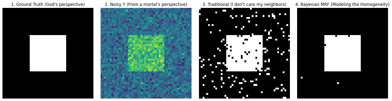
axes[0].set_title("1. Ground Truth (God's perspective)")
axes[0].axis('off')

axes[1].imshow(Y, cmap='viridis')
axes[1].set_title("2. Noisy Y (From a mortal's perspective)")
axes[1].axis('off')

axes[2].imshow(L_traditional, cmap='gray')
axes[2].set_title("3. Traditional (I don't care my neighbors)")
axes[2].axis('off')

axes[3].imshow(L_mrf, cmap='gray')
axes[3].set_title("4. Bayesian MRF (Modeling the Homogeneity)")
axes[3].axis('off')

plt.tight_layout()
plt.show()

🚀 Starting Bayesian MRF Optimization Engine...
Iteration 1/15 Complete | Temp T = 3.00
Iteration 2/15 Complete | Temp T = 2.35
Iteration 3/15 Complete | Temp T = 1.85
Iteration 4/15 Complete | Temp T = 1.45
Iteration 5/15 Complete | Temp T = 1.14
Iteration 6/15 Complete | Temp T = 0.89
Iteration 7/15 Complete | Temp T = 0.70
Iteration 8/15 Complete | Temp T = 0.55
Iteration 9/15 Complete | Temp T = 0.43
Iteration 10/15 Complete | Temp T = 0.34
Iteration 11/15 Complete | Temp T = 0.26
Iteration 12/15 Complete | Temp T = 0.21
Iteration 13/15 Complete | Temp T = 0.16
Iteration 14/15 Complete | Temp T = 0.13
Iteration 15/15 Complete | Temp T = 0.10

Look closely at the images above:

• Image 3 (Traditional Method): Because it assumes pixels are absolutely independent, it is completely deceived by Gaussian noise, resulting in “snowflakes” of misclassification.
• Image 4 (Bayesian MRF): A miracle! Under the “homogeneity prior” imposed by penalty coefficient and the step-by-step approach of simulated annealing, the system forcefully “washes away” those isolated noise points one by one. It not only perfectly recovers the clear boundary of the square but also retrieves that clean, smooth visual aesthetic.

This is the masterpiece woven by Bayesian Statistics and Markov Random Fields (MRF)!

Ultimate Practice — Understanding Bayesian MRF through “Black Cat” Segmentation

In previous sections, we derived profound formulas and demonstrated principles with minimal code. Now, it’s time for a real battle.

The goal is to extract a “Black Cat” (Foreground, Label 1) from the background (Label 2) in a noisy image.

In real images, background and foreground colors are not black and white; they follow Gaussian Distributions. We calculate mean and standard deviation for each category based on training samples:

• Black cat mean is darker $\mu_1 = 19$, variance $\sigma_1 = 23$;
• Background is brighter $\mu_2 = 209$, variance $\sigma_2 = 29$.

We compare three methods for image segmentation:

Method 1: Naive Maximum Likelihood Estimation

This is the simplest method. It completely ignores spatial relationships between pixels. For each pixel, it calculates: what is the Gaussian probability if this pixel belongs to the black cat? What if it belongs to the background? Choose whichever is larger.

• Expected Result: Image filled with “snowflake” noise.

Method 2: MRF + Simulated Annealing + Gibbs Sampling (Stochastic)

It takes into account the local Markov property (MRF) of pixels. Based on the formula in the code, the conditional probability $p_T(x_i | x_{-i}, y)$ of pixel $x_i$ is converted into an elegant energy function:

• First and Second Terms: Data Term (Likelihood), punishing colors that do not fit the Gaussian distribution.
• Third Term: Smoothness Term (Prior), strongly requiring the current pixel to be consistent with surrounding neighbors via penalty coefficient $\alpha$ (set to a striking 30 in code).

Then, using simulated annealing to cool from high to low temperature, combined with Gibbs sampling dice rolling, we finally obtain the perfect solution.

Method 3: Simple Relaxation (ICM)

Simulated annealing is good, but because it involves dice rolling (random sampling), it is relatively slow.

Therefore, one of the compromise solutions commonly used in industry is: Simple Relaxation (usually called ICM, Iterated Conditional Modes in academia). Its calculation formula is exactly the same as Method 2, but it does not roll dice! When updating each pixel, it directly greedily selects the label that minimizes energy (maximizes probability). After a few iterations, once the image no longer changes, it stops immediately.

Python Practice: Code Battle of Three Methods

In the code below, we first automatically generate a “synthetic black cat” with Gaussian noise, and then segment it using these three methods respectively.

⚠️ Core Code Highlight:

Note the Log-Sum-Exp Trick in the MRF_Gibbs_SA function. When energy values are high, directly calculating $e^{-\text{Energy}}$ causes computer numerical underflow (becoming 0). We subtract the maximum value lnA = -max(...) for numerical regularization. This is valuable engineering experience!

import numpy as np
import matplotlib.pyplot as plt

# ==========================================
# 0. Data Prep: Generate "Synthetic Black Cat" Noisy Image
# ==========================================
rows, cols = 80, 80
true_L = np.ones((rows, cols), dtype=int) * 2 # Background Label 2
# Draw an "Abstract Black Cat" in center (Label 1)
true_L[20:60, 30:50] = 1 
true_L[15:20, 30:35] = 1 # Left Ear
true_L[15:20, 45:50] = 1 # Right Ear

# True Gaussian params (Ref MATLAB settings)
mu_x = {1: 100.0, 2: 180.0}      # 1:Cat(Dark), 2:Background(Bright)
sigma_x = {1: 30.0, 2: 30.0}

# Add Gaussian Noise to generate Y
Y = np.zeros_like(true_L, dtype=float)
for r in range(rows):
    for c in range(cols):
        label = true_L[r, c]
        Y[r, c] = np.random.normal(mu_x[label], sigma_x[label])

# Clip pixel values to 0~255
Y = np.clip(Y, 0, 255)

# ==========================================
# Level 1: Naive Maximum Likelihood (No MRF)
# ==========================================
def maximum_likelihood(Y):
    L_ml = np.zeros_like(Y, dtype=int)
    # Calculate Likelihood Energy for 1 and 2 (Data term only)
    for r in range(rows):
        for c in range(cols):
            # Energy = log(sigma) + (y - mu)^2 / (2*sigma^2)
            E1 = np.log(sigma_x[1]) + (Y[r, c] - mu_x[1])**2 / (2 * sigma_x[1]**2)
            E2 = np.log(sigma_x[2]) + (Y[r, c] - mu_x[2])**2 / (2 * sigma_x[2]**2)
            L_ml[r, c] = 1 if E1 < E2 else 2 # Choose lower energy
    return L_ml

# ==========================================
# Level 2: MRF + Simulated Annealing + Gibbs Sampling
# ==========================================
def mrf_simulated_annealing(Y, initial_L, alpha=30, iter_max=50, Tin=100, Tend=0.01):
    L = np.copy(initial_L)
    tau = -np.log(Tend / Tin) / (iter_max - 1)
    
    for it in range(iter_max):
        T = Tin * np.exp(-tau * it)
        padded_L = np.pad(L, 1, mode='edge')
        
        for r in range(1, rows + 1):
            for c in range(1, cols + 1):
                neighbors = [padded_L[r-1, c], padded_L[r+1, c], padded_L[r, c-1], padded_L[r, c+1]]
                
                pt_xi = {}
                for k in [1, 2]:
                    # Total Energy = Data + Smoothness
                    E_data = np.log(sigma_x[k]) + (Y[r-1, c-1] - mu_x[k])**2 / (2 * sigma_x[k]**2)
                    E_smooth = alpha * sum([abs(k - n) for n in neighbors])
                    # Gibbs Probability Exponent
                    pt_xi[k] = - (1.0 / T) * (E_data + E_smooth)
                
                # [Engineering Trick] Numerical Regularization: Prevent overflow
                max_pt = max(pt_xi[1], pt_xi[2])
                p1 = np.exp(pt_xi[1] - max_pt)
                p2 = np.exp(pt_xi[2] - max_pt)
                
                # Normalize to probability and roll dice
                prob_1 = p1 / (p1 + p2)
                padded_L[r, c] = 1 if np.random.rand() < prob_1 else 2
                
        L = padded_L[1:-1, 1:-1]
    return L

# ==========================================
# Level 3: Simple Relaxation (ICM)
# ==========================================
def simple_relaxation(Y, initial_L, alpha=30, iter_max=50):
    L = np.copy(initial_L)
    
    for it in range(iter_max):
        L_prec = np.copy(L)
        padded_L = np.pad(L, 1, mode='edge')
        
        for r in range(1, rows + 1):
            for c in range(1, cols + 1):
                neighbors = [padded_L[r-1, c], padded_L[r+1, c], padded_L[r, c-1], padded_L[r, c+1]]
                
                E = {}
                for k in [1, 2]:
                    E_data = np.log(sigma_x[k]) + (Y[r-1, c-1] - mu_x[k])**2 / (2 * sigma_x[k]**2)
                    E_smooth = alpha * sum([abs(k - n) for n in neighbors])
                    # Relaxation doesn't need divide by T
                    E[k] = E_data + E_smooth
                
                # [Core Difference] No dice, Greedy choice
                padded_L[r, c] = 1 if E[1] < E[2] else 2
                
        L = padded_L[1:-1, 1:-1]
        
        # Early Stopping
        if np.sum(np.abs(L_prec - L)) == 0:
            print(f"Simple Relaxation converged at iteration {it+1}!")
            break
            
    return L

# Run Comparison
print("1. Computing Max Likelihood...")
L_ml = maximum_likelihood(Y)

print("2. Running MRF Simulated Annealing...")
L_sa = mrf_simulated_annealing(Y, initial_L=L_ml, alpha=1.5)

print("3. Running MRF Simple Relaxation...")
L_sr = simple_relaxation(Y, initial_L=L_ml, alpha=1.5)

# Visualize Results
fig, axes = plt.subplots(1, 5, figsize=(18, 4))
titles = ["1. Ground Truth", "2. Noisy Y", "3. Maximum Likelihood", "4. MRF + SA (Stochastic)", "5. MRF + SR (Deterministic)"]
images = [true_L, Y, L_ml, L_sa, L_sr]

for ax, img, title in zip(axes, images, titles):
    ax.imshow(img, cmap='gray' if title != "2. Noisy Y" else 'viridis')
    ax.set_title(title)
    ax.axis('off')

plt.tight_layout()
plt.show()

1. Computing Max Likelihood...
2. Running MRF Simulated Annealing...
3. Running MRF Simple Relaxation...
Simple Relaxation converged at iteration 3!

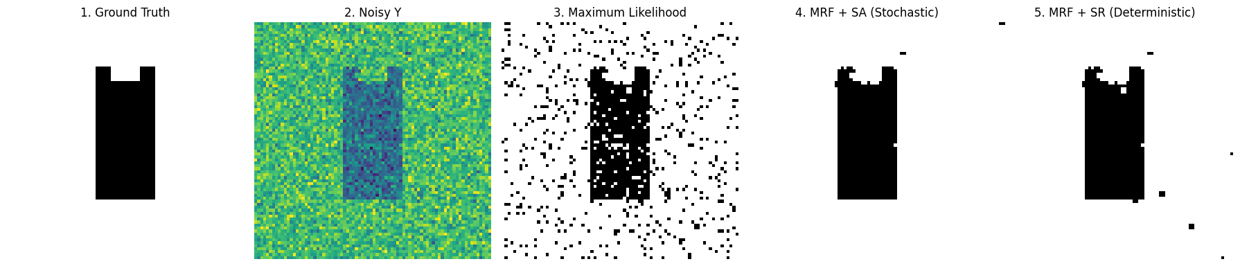
Look at the 5 comparison images above:

• Image 3 (Max Likelihood): Like a poor quality black and white newspaper, full of white noise. This is the cost of abandoning spatial priors.
• Image 4 (Simulated Annealing SA): Perfectly restores the shape of the black cat. Because it went through high-temperature annealing, it successfully jumped out of local optimal traps.
• Image 5 (Simple Relaxation SR): Extremely fast, also restores outline. But because it’s too greedy (rejects worsening results), the edges are often less smooth than SA, and sometimes it gets stuck in dead ends.

Ultimate Easter Egg: The Golden Partner in Industry — “Stochastic Coarse Tuning” + “Deterministic Fine Tuning”

After running the code above, you might have a question: Since Simulated Annealing (SA) is so powerful, why do we still need ICM (Simple Relaxation)?

This touches on a core pain point in algorithm engineering: Stochastic (random algorithms) usually only get an “approximate optimal solution,” but cannot achieve “absolute optimal.”

Why is SA only “Approximate”?

• Theoretically, Simulated Annealing can find the global optimum, but only if “time is infinite and cooling is infinitely slow.”
• In actual coding, to make the program finish in seconds, our cooling steps (iter_max) are usually limited, and the cooling rate is compromised. This results in the temperature $T$ not truly reaching absolute 0 at the end of iteration.
• As long as $T > 0$, Gibbs sampling always has “dice rolling” randomness. It might jump back and forth (Jittering) near the global optimal solution, giving you a result $99\%$ close to perfect, but can never completely lock onto that absolute bottom.

Why is ICM a “Dangerous Fast Knife”?

• ICM (Simple Relaxation) is Deterministic. It rolls no dice, extremely greedy: as long as energy drops, it goes there without hesitation; once there’s no way to go, it stops immediately.
• Its advantage is extremely fast convergence and can reach absolute local optimal; disadvantage is narrow vision, if the starting point is bad, it instantly falls into a wrong “local dead end.”

Ultimate Logic: Mixed Doubles (Stochastic + Deterministic)

Since they each have pros and cons, why not combine them? This gives birth to the ultimate paradigm of MRF optimization: SA for Coarse Tuning first, then ICM for Fine Tuning.

It’s like playing golf:

1. First Shot (Simulated Annealing SA): Big power for miracles. Use its randomness and jumping ability to cross various local traps and hit the ball very close to the hole on the green (Find Approximate Optimal).
2. Second Shot (Simple Relaxation ICM): Precision putting. Use the approximate solution from SA as the starting point, use its greedy, deterministic nature to hole in one, eliminating the last bit of random noise, and steadily land in the lowest energy point (Lock Absolute Optimal).

Python Practice: Completing this “Combo”

In code implementation, this combo is extremely simple, just feed the output of SA as the input start point for ICM.

# ==========================================
# Ultimate Combo: Hybrid Optimization (SA -> ICM)
# ==========================================

print("🚀 Step 1: Start Simulated Annealing (SA) for Global Coarse Tuning...")
# Run SA a bit, no need for too many iterations, wash away large noise areas, find rough pit bottom
L_approx_opt = mrf_simulated_annealing(Y, initial_L=L_ml, alpha=5.0, iter_max=30)

print("🎯 Step 2: Start Simple Relaxation (ICM) for Local Fine Tuning...")
# Feed SA result (L_approx_opt) directly to ICM as start point (initial_L)
L_absolute_opt = simple_relaxation(Y, initial_L=L_approx_opt, alpha=5.0, iter_max=20)

print("✅ Optimization Implemented! We got the absolute optimal MAP.")

🚀 Step 1: Start Simulated Annealing (SA) for Global Coarse Tuning...
🎯 Step 2: Start Simple Relaxation (ICM) for Local Fine Tuning...
Simple Relaxation converged at iteration 1!
✅ Optimization Implemented! We got the absolute optimal MAP.

Principle Analysis: Because SA has already eliminated all “wrong traps” for ICM and sent it to the door of the global optimal solution. Starting ICM at this time, its greedy and deterministic downhill ability acts like gravity, completely flattening the last few “restless pixels” caused by SA randomness, instantly achieving $100\%$ convergence.

This is the real Master Class Technique when solving complex non-convex optimization problems!

See also

• Markov Random Fields (MRF)
• Stochastic Optimization Explained: Simulated Annealing & Pincus Theorem
• Deterministic Optimization Explained: The Mathematical Essence of Gradient Descent
• Gibbs Sampling Explained: The Wisdom of Divide and Conquer
• Metropolis Algorithm Explained: Implementation & Intuition