🏷️ Model Name
MAE – Masked Autoencoders Are Scalable Vision Learners
🧠 Core Idea
Randomly mask image patches and reconstruct the missing ones to learn context-aware visual representations.
🖼️ Architecture
                +-----------------------+
                |     Input Image       |
                +-----------------------+
                            |
                            v
                +-----------------------+
                | Patch Embedding (ViT) |
                +-----------------------+
                            |
                |-----------------------------|
                |  Random Masking (e.g. 75%)  |
                |-----------------------------|
                            |
                            v
                +-----------------------+
                |     Encoder (ViT)     |   <-- only visible patches
                +-----------------------+
                            |
                            v
                +-----------------------+
                | Add Mask Tokens + Pos |
                +-----------------------+
                            |
                            v
                +-----------------------+
                |     Decoder (ViT)     |   <-- lightweight
                +-----------------------+
                            |
                            v
                +-----------------------+
                |  Reconstructed Image  |
                +-----------------------+
                            |
                            v
                +-----------------------+
                |     MSE Loss          |
                +-----------------------+
And the pseudocode:
for image in dataloader:
    patches = patchify(image) # Divide image into patches
    visible, masked = random_mask(patches, ratio=0.75) # Randomly mask 75% patches.

    latent = encoder(visible) # Feed visible patches into encoder.
    full_tokens = fill_with_mask_tokens(latent, masked)

    reconstructed = decoder(full_tokens) # Reconstruct all patches using a lightweight decoder.
    loss = mse_loss(reconstructed[masked], patches[masked]) # Compute loss between reconstructed and original patches.

    # Backpropagate through encoder + decoder.
    loss.backward()
    update(encoder, decoder)
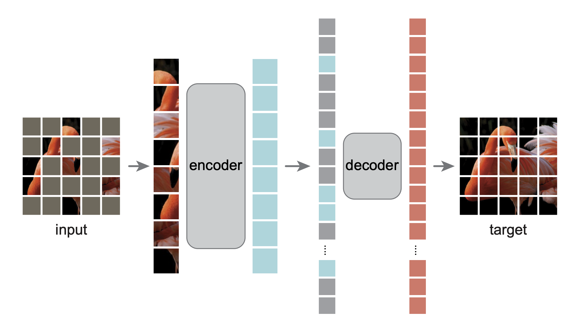
1️⃣ Image Patching and Masking
- Divide the image into patches: The input image is first divided into regular, non-overlapping patches, similar to the approach used in Vision Transformers (ViT).
- Apply masking: A large random subset of these patches is sampled and removed (masked out). This random sampling is typically performed without replacement, following a uniform distribution. Crucially, MAE usually employs a very high masking ratio, such as 75%, to reduce redundancy and force the model to learn holistic understanding rather than relying on low-level statistics.
2️⃣ MAE Encoder Processing
The MAE encoder, which is a
The visible patches are first mapped via a
By having the encoder process only 25% (or less) of the input patches, the pre-training time is greatly reduced (e.g., 3× or more speedup) and memory consumption is lowered.
3️⃣ Decoder Input Preparation
- Reintroduce missing patches: After the encoder processes the visible patches, the encoded visible patches are combined with a set of mask tokens. Each mask token is a shared, learned vector used to indicate the presence of a missing patch that needs to be predicted.
- Add positional information: Positional embeddings are added to all tokens in this full set (both the encoded visible patches and the mask tokens) so that the mask tokens receive information about their location in the original image. The encoder output may pass through a linear projection layer to match the decoder’s width.
4️⃣ MAE Decoder Reconstruction
The full set of tokens (encoded patches + mask tokens) is processed by the MAE decoder, which consists of another series of Transformer blocks.
- Asymmetric design: The decoder is intentionally designed to be lightweight (narrower and shallower than the encoder), for instance, having 8 blocks and a 512-dimensional width, accounting for a small fraction of the overall compute (e.g., <10% computation per token vs. the encoder).
- Reconstruct pixels: The decoder performs the reconstruction task by predicting the pixel values for each masked patch. The final layer of the decoder is a linear projection, yielding a vector of pixel values for each patch. The decoder output is then reshaped to form the reconstructed image.
5️⃣ Loss Calculation
- Define reconstruction target: The reconstruction target is typically the pixel values of the original image. Using normalized pixel values (where the mean and standard deviation are computed per patch) often improves the quality of the learned representation.
- Compute loss: The MAE uses the
mean squared error (MSE) as its loss function, which is computed only on the masked patches.
🎉 Deployment
- Discard the decoder: After the self-supervised pre-training is finished, the decoder component is discarded.
- Use the encoder: The encoder is retained and applied to uncorrupted images (the full set of patches) to extract features for various downstream recognition tasks, such as fine-tuning a classifier.
🎯 Downstream Tasks
- Image Classification: Evaluated via end-to-end fine-tuning on ImageNet-1K and using linear probing on frozen features.
- Object Detection: Transfer learning, typically fine-tuned on datasets such as COCO and PASCAL VOC.
- Instance Segmentation: Transfer learning, evaluated on datasets like COCO.
- Semantic Segmentation: Transfer learning, evaluated on datasets like ADE20K using UperNet.
- Transfer Classification Tasks: Fine-tuning on diverse classification datasets, including iNaturalists and Places (e.g., Places205, Places365).
- Model Robustness: Evaluating performance on corrupted or modified image datasets (e.g., IN-Corruption, IN-Adversarial).
- Low-Level Tasks: Masked Image Modeling (MIM), the paradigm MAE belongs to, is suitable for tasks such as denoising and superresolution.
💡 Strengths
- Training Efficiency and Scalability
- High Training Speed: MAE significantly accelerates training, achieving a speedup of 3x or more in pre-training time due to its asymmetric design. Wall-clock speedups can range from 2.8x to 4.1x for large models.
- Reduced Computation and Memory: The asymmetric architecture mandates that the encoder only processes the small subset of visible patches, leading to a large reduction in computation and lowering memory consumption. The overall training FLOPs can be reduced by 3.3x.
- Scalable Architecture: MAE is a scalable self-supervised learner that efficiently enables the training of very large models such as ViT-Huge.
- Simplicity of Implementation: The approach is conceptually simple, effective, and scalable. It does not require specialized sparse operations, and the pixel-based reconstruction target is much simpler than tokenization methods like BEiT.
- Superior Performance and Generalization
- State-of-the-Art Accuracy: MAE pre-training enables high-capacity models to generalize well. A vanilla ViT-Huge model achieved the best reported accuracy (87.8% Top-1) among methods using only ImageNet-1K data.
- Improved Transferability: Transfer performance on downstream tasks (e.g., object detection, instance segmentation, semantic segmentation) outperforms supervised pre-training.
- Scaling Gains: MAE shows strong scaling behavior, with generalization gains increasing significantly as model capacity grows, following a trend similar to models supervisedly pre-trained on massive datasets (like JFT-300M).
- Architectural and Training Robustness
- Tolerance to High Masking: Masking a very high proportion of random patches (e.g., 75%) yields a non-trivial and meaningful self-supervisory task, which is crucial for reducing image redundancy and forcing holistic understanding.
- Minimal Data Augmentation Required: The framework works well with minimal or no data augmentation (only cropping/resizing), unlike contrastive methods that heavily rely on complex augmentations (like color jittering) for regularization.
- Effective Non-Linear Features: MAE produces stronger non-linear features compared to contrastive methods (like MoCo v3). Fine-tuning just the last one or two Transformer blocks can yield significant accuracy gains beyond linear probing.
- Flexibility of Decoder: The decoder is lightweight (e.g., <10% computation per token vs. the encoder) and flexible in its design.
⚠️ Limitations
- Weakness in Linear Separability
Low Linear Probing Accuracy : MAE representations are generally less linearly separable. The accuracy obtained via the linear probing protocol is typically lower than that achieved by contrastive methods (like MoCo v3).Lack of Correlation with Fine-Tuning : Linear probing results are largely uncorrelated with end-to-end fine-tuning results.Dependency on Decoder Depth (for linear probing) : Achieving high linear probing accuracy requires a sufficiently deep decoder to ensure the learned latent representations remain at a high abstract level, rather than specializing too much on pixel reconstruction.
- Architectural Constraints and Task Suitability
ViT Dependency : Masked Image Modeling (MIM) approaches, including MAE, require a ViT backbone because the method is based on processing sequential patches. This contrasts with Joint Embedding approaches which are architecture agnostic.Lower Semantic Level of Reconstruction : Reconstructing raw pixels means the decoder output is often considered of a lower semantic level compared to the high-level semantic information generated in language models (e.g., predicting words in BERT).Qualitative Reconstruction Issues : Since the loss is computed only on masked patches, the model output on visible patches is qualitatively worse in reconstructions.Masking Strategy Sensitivity : While random sampling works best, the model is susceptible to poorer performance if less effective masking strategies, such as block-wise masking, are used at high ratios.
📚 Reference
- He et al., 2022 [Masked Autoencoders Are Scalable Vision Learners] 🔗 arXiv:2111.06377
- Github: facebookresearch/mae
Scan to Share
微信扫一扫分享