title: “BYOL Explained: Self-Supervised Learning without Negative Pairs” date: 2025-10-08 summary: “Understanding BYOL: How interactions between Online and Target networks achieve SOTA performance without negative samples. A deep dive into the architecture and loss function.” series: [“Self-Supervised Learning”] tags: [“BYOL”, “Contrastive Learning”, “SSL”, “CV”, “Paper Notes”]
🏷️ Model Name
BYOL – Bootstrap Your Own Latent
🧠 Core Idea
Two interacting neural networks—the
online network and thetarget network —— learn representations by predicting each other’s outputs, without using negative samples.Objective: train the online network to
predict the target network’s projection of the same image under a different augmented view.
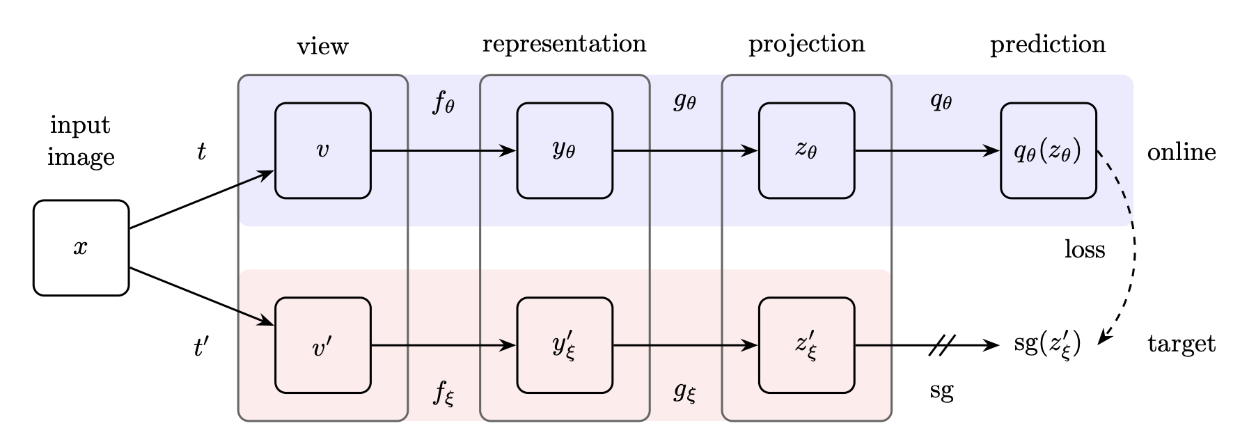
🖼️ Architecture
BYOL employs two parallel neural networks: the online network (parameters $\theta$) and the target network (parameters $\xi$).
Online Network $(\theta)$: This network is comprised of three sequential stages:- An encoder ($f_{\theta}$): a convolutional neural network (such as
ResNet ) used to extract image feature representation $y_{\theta}$. - A projector ($g_{\theta}$): a
multi-layer perceptron (MLP) projecting the encoder output $y_{\theta}$ into a smaller latent space to obtain the projection $z_{\theta}$. - A predictor ($q_{\theta}$): another
MLP , with the same structure as the projector, is used to predict the projection of the target network.
- An encoder ($f_{\theta}$): a convolutional neural network (such as
Target Network $(\xi)$: This network has the same encoder ($f_{\xi}$) and projector ($g_{\xi}$) architecture as the online network, but it does not have a predictor. The target network weights $\xi$ are initialized to match the online network weights $\theta$.
And the pseudocode of BYOL’s main learning algorithm:
1️⃣ Data Augmentation and View Generation
- An input image ($x$) is sampled from the dataset.
- Two distributions of image augmentations, $T$ and $T'$, are used to create two different augmented views of the image: $v = t(x)$ and $v' = t'(x)$, where $t \sim T$ and $t' \sim T'$.
- The augmentations typically include random cropping/resizing, random horizontal flip, color distortion, Gaussian blur, and solarization.
2️⃣ Forward Pass through Online and Target Branches
The two augmented views, $v$ and $v'$, are processed by the two distinct networks:
- Online Branch (View $v$):
- The encoder $f_{\theta}$ processes $v$ to yield the representation $y_{\theta}$.
- The projector $g_{\theta}$ maps $y_{\theta}$ to the projection $z_{\theta}$.
- The predictor $q_{\theta}$ transforms $z_{\theta}$ to generate the prediction $q_{\theta}(z_{\theta})$.
- Target Branch (View $v'$):
- The encoder $f_{\xi}$ processes $v'$ to yield the representation $y'_{\xi}$.
- The projector $g_{\xi}$ maps $y'_{\xi}$ to the target projection $z'_{\xi}$.
3️⃣ Loss Calculation
The objective is to train the online network to predict the target network’s output:
- Normalization: Both the prediction $q_{\theta}(z_{\theta})$ and the target projection $z'_{\xi}$ are $\ell_2$-normalized.
- Stop Gradient: A stop-gradient operator (sg) is applied to the target projection $z'_{\xi}$, ensuring that the gradient does not propagate back into the target network parameters $\xi$.
- Loss Definition: The loss ($L_{\theta, \xi}$) is defined as the mean squared error (MSE) between the normalized prediction and the normalized target projection: $$L_{\theta, \xi} = \left\| q_{\theta}(z_{\theta}) - z'_{\xi} \right\|_2^2$$.
- Symmetrization: The total BYOL loss ($L_{\text{BYOL}}$) is symmetrized by repeating the process with the inputs swapped (i.e., feeding $v'$ to the online network and $v$ to the target network to compute $\tilde{L}_{\theta, \xi}$): $$L{\text{BYOL}} = L_{\theta, \xi} + \tilde{L}_{\theta, \xi}$$.
4️⃣ Parameter Update
The two networks are updated differently in an asymmetric manner:
- Online Network Update ($\theta$): The online parameters $\theta$ are updated by
a stochastic optimization step (e.g., using the LARS optimizer) to minimize $L_{\text{BYOL}}$. - Target Network Update ($\xi$): The target parameters $\xi$ are updated using an
Exponential Moving Average (EMA) of the online parameters $\theta$. This update is slow and steady, calculated as: $$\xi \leftarrow \tau\xi + (1-\tau)\theta$$ where $\tau \in$ is the momentum coefficient (often starting from $\tau_{\text{base}}=0.996$ and increasing to one). This EMA mechanism is crucial for stabilizing the bootstrap targets.
🎉 Final Output
After the self-supervised training is complete, everything except the encoder $f_{\theta}$ is discarded, and $f_{\theta}$ provides the learned image representation for downstream tasks.
🎯 Downstream Tasks
- ImageNet Evaluation Protocols
- Transfer Learning Tasks (General Vision)
- Classification (Transfer to other classification tasks).
- Semantic Segmentation (e.g., VOC2012 task).
- Object Detection (Using architectures like Faster R-CNN).
- Depth Estimation (e.g., NYU v2 dataset).
💡 Strengths
- Performance and Efficiency
- State-of-the-Art Performance Without Negatives: BYOL achieves state-of-the-art results without relying on negative pairs.
- High Accuracy.
- Outperforms on Transfer Benchmarks
- Parameter Efficiency
- Simple and Powerful Objective
- Robustness and Training Flexibility
- Insensitivity to Batch Size: BYOL is more resilient to changes in the batch size compared to contrastive counterparts. Its performance remains stable over a wide range of batch sizes (from 256 to 4096), only dropping for very small values due to reliance on batch normalization layers.
- No Need for Large Batches: Since it does not rely on negative pairs, there is no need for large batches of negative samples.
- Robustness to Augmentations: BYOL is incredibly robust to the choice of image augmentations compared to contrastive methods like SimCLR. When augmentations are drastically reduced to only random crops, BYOL shows much smaller performance degradation than SimCLR.
- Effective Use of Moving Average Target: The use of a slow-moving exponential average (EMA) of the online network parameters for the target network provides stable targets, which is crucial for stabilizing the bootstrap step.
⚠️ Limitations
- Theoretical and Architectural Constraints
Susceptibility to Collapse : The core objective of BYOL—predicting the target network’s output—theoretically admits collapsed solutions (where the network outputs the same vector for all inputs). While BYOL employs specific mechanisms (predictor, EMA target) to avoid this, distillation methods generally are noted as being more prone to collapsing.Dependence on Asymmetry : The design requires an asymmetric architecture, specifically the addition of a predictor ($q_{\theta}$) to the online network, which is critical to preventing collapse in the unsupervised scenario. If this predictor is removed, the representation collapses.
- Generalization Constraints
Dependence on Vision-Specific Augmentations : BYOL remains dependent on existing sets of augmentations that are specific to vision applications.Generalization Difficulty to Other Modalities : Generalizing BYOL to other modalities (e.g., audio, video, text) would require significant effort and expertise to design similarly suitable augmentations for each modality.
📚 Reference
- Grill et al., 2020 [Bootstrap Your Own Latent: A New Approach to Self-Supervised Learning] 🔗 arXiv:2006.07733
- Github: BYOL
- Github: deepmancer/byol-pytorch
Scan to Share
微信扫一扫分享